Spearman Rank Correlation
For completeness, I’m going to briefly mention Spearman rank correlation as well. At a conceptual level, it’s the same idea as Pearson similarity, but instead of using rating scores directly we use ranks instead. That is, instead of using an average rating value for a movie, we’d use its rank amongst all movies based on their average ratings. And instead of individual ratings for a movie, we’d rank that movie amongst all that individuals’ ratings.
I’m not going into the details on this, because it’s going to confuse you. The math gets tricky, it’s very computationally intensive, and it’s generally not worth it. The main advantage of Spearman is that it can deal with ordinal data effectively, for example if you had a rating scale where the difference in meaning between different rating values were not the same. I’ve never seen this actually used in real world applications myself, but you may encounter it in the academic literature
.
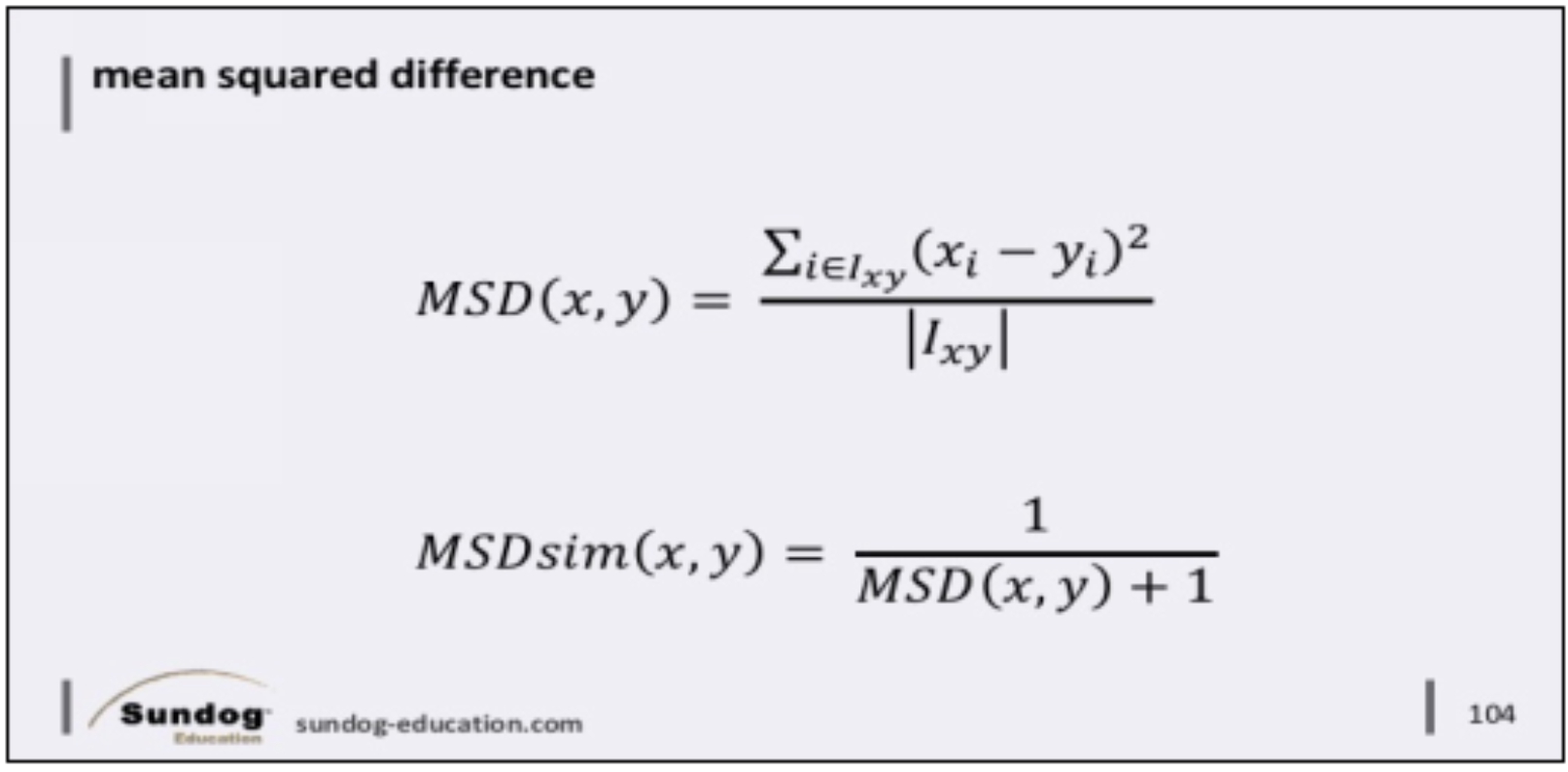
Mean Squared Difference
Another way to measure similarity is the mean squared difference similarity metric, and it’s exactly what it sounds like. You look at, say, all of the items that two users have in common in their ratings, and compute the mean of the squared differences between how each user rated each item. It’s easier to wrap your head around this, since it doesn’t involve angles in multi-dimensional space – you’re just directly comparing how two people rated the same set of things. It’s very much the same idea of how we measure mean absolute error when measuring the accuracy of a recommender system as a whole.
So if we break down that top equation, it says the mean squared difference, or MSD for short, between two users X and Y, is given by the following. On the top of this fraction, we are summing up for every item I that users X and Y have both rated, the difference between the ratings from each user, squared. We then divide by the number of items these users had in common that we summed across, to get the average, or mean
.
Now the problem is that we’ve computed a metric of how different users x and y are, and we want a measure of how similar they are, not how different they are. So to do that, we just take the inverse of MSD, dividing it by one – and we have to stick that “plus one” on the bottom in order to avoid dividing by zero in the case where these two users have identical rating behavior.
You can, by the way, flip everything we just said to apply to items instead of users. So, x and y could refer to two different things instead of two different people, and then we’d be looking at the differences in ratings from the people these items have in common, instead of the items people have in common. As we’ll see shortly, there are two different ways of doing collaborative filtering – item-based, and user-based, and it’s important to remember that most of these similarity metrics can apply to either approach.
So that’s MSD. It’s easier to comprehend than cosine similarity metrics, but in practice you’ll usually find that cosine works better.