So if we look at the data we’re working with in the Iris data set, we have length and width of petals and sepals for each Iris we’ve measured – so that’s a total of four dimensions of data.
Our feeble human brains can’t picture a plot of 4D data, so let’s just think about the petal length and width at first. That’s plotted here for all of the irises in our data set.
Without getting into the mathematical details of how it works, those black arrows are what’s called the “eigenvectors” of this data. Basically, it’s the vector that can best describe the variance in the data, and the vector orthogonal to it. Together, they can define a new vector space, or basis, that better fits the data.
These eigenvectors are our “principal components” of the data. That’s why it’s called principal component analysis – we are trying to find these principal components that describe our data, which are given by these eigenvectors
.
Let’s think about why these principal components are useful. First of all, we can just look at the variance of the data from that eigenvector. That distance from the eigenvector is a single number; a single dimension that is pretty good at reconstructing the two-dimensional data we started with here for petal length and petal width. So you can see how identifying these principal components can let us represent data using fewer dimensions than we started with.
Also, these eigenvectors have a way of finding interesting features that are inherent in the data. In this case, we’re basically discovering that the overall size of an iris’s petals are what’s important for classifying which species of iris it is, and the ratio of width to length is more or less constant. So the distance along this eigenvector is basically measuring the “bigness” of the flower. The math has no idea what “bigness” means, but it found the vector that defines some hidden feature in the data that seems to be important in describing it – and it happens to correspond to what we call “bigness.”
So, we can also think of PCA as a feature extraction tool. We call the features it discovers latent features.
So here’s what the final result of PCA looks like on our complete 4-dimensional Iris data set – we’ve used PCA to identify the two dimensions within that 4-D space that best represents the data, and plotted it in those two dimensions. PCA by itself will give you back as many dimensions as you started with, but you can choose to discard the dimensions that contain the least amount of information. So by discarding the two dimensions from PCA that told us the least about our data, we could go from 4 dimensions down to 2.
We can’t really say what these two dimensions represent. What does the X axis in this plot mean? What does the Y axis mean? All we know for sure is
that they represent some sort of latent factors, or features, that PCA extracted from the data. They mean something, but only by examining the data can we attempt to put some sort of human label on them.
So just like we can run PCA on a 4-dimensional Iris data set, we can also run it on our multidimensional movie rating data set, where every dimension is a movie. We’ll call this ratings matrix that has users as rows R.
Just like it did with our Iris data set, PCA can boil this down to a much smaller number of dimensions that best describe the variance in the data. And often, the dimensions it finds correspond to features humans have learned to associate with movies as well, for example, how “action-y” is a movie? How romantic is it? How funny is it? Whatever it is about movies that causes individuals to rate them differently, PCA will find those latent features and extract them from the data. PCA doesn’t know what they mean, but it finds them nonetheless.
So, we could ask PCA to distill things down to say 3 dimensions in this example, and it would boil our ratings down to 3 latent features it identified.
PCA won’t know what to call them, but let’s say they end up being measures of each person’s interest in action, sci-fi, and classic genres. So for example, we might think of Bob as being defined as 30% action, 50% sci-fi, and 20% classic in terms of his interests.
Now, take a look at the columns in this new matrix. Each column is a description of users that make up that feature. “Action” can be described as 30% of Bob plus 10% of Ted plus 30% of Ann.
Let’s call this matrix U – its columns describe typical users for each latent feature we produced.
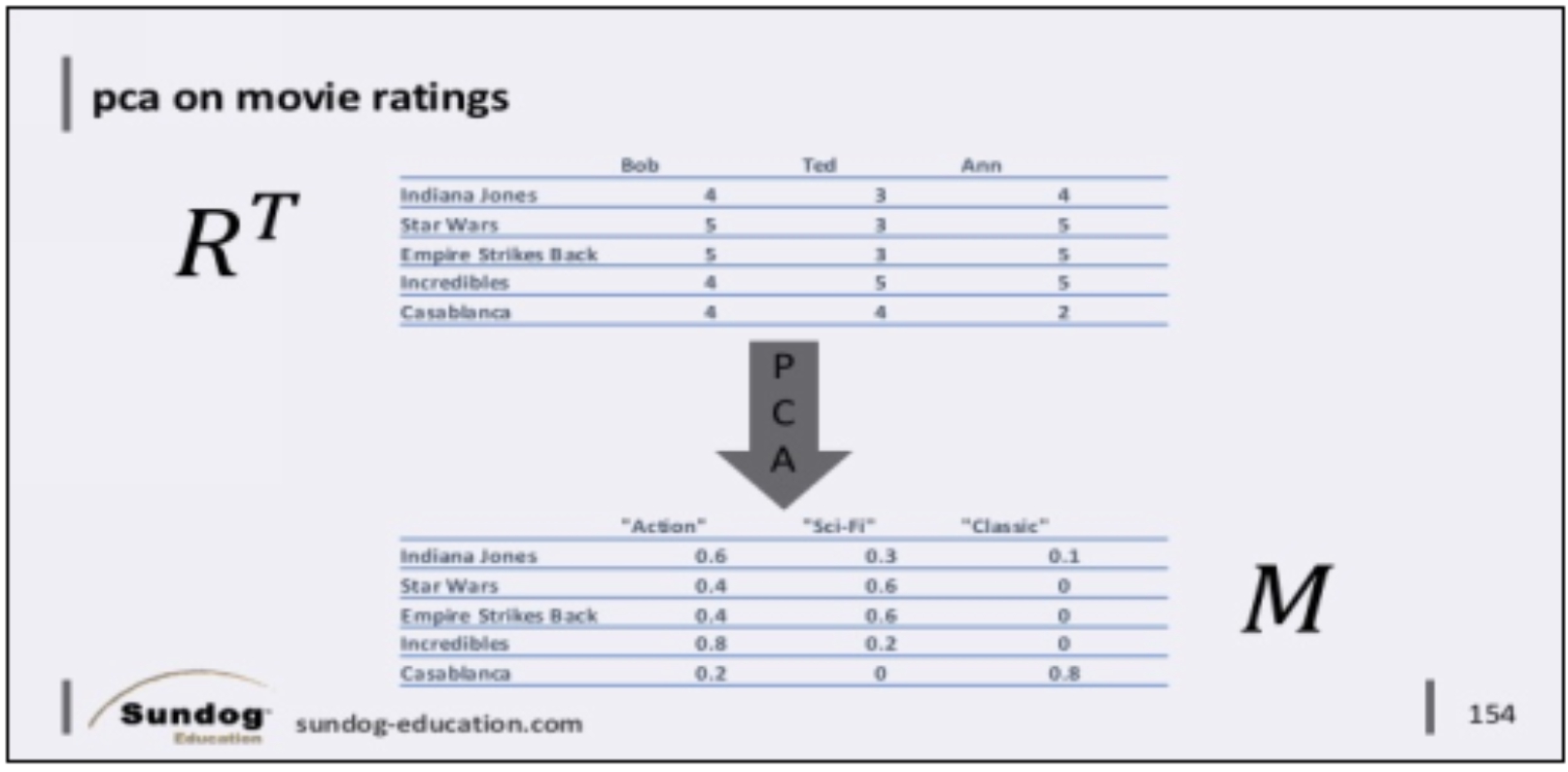
Just like we can run PCA on our user ratings data to find profiles of typical kinds of users, we can flip things around and run PCA to find profiles of typical kinds of movies.
If we re-arrange our input data so that movies are rows and users are columns, it would look like this. We call this the transpose of the original ratings matrix, or R-T for short
.
Now if we run PCA on that, it will identify the latent features again, and describe each individual movie as some combination of them. Each column is now a description of some typical movie that exhibits some latent feature. Again, these have no inherent meaning, but in practice it might fall along movie genre lines – in reality though, it’s more complex.
 Let’s call this resulting matrix that describes typical movies M.
So how do these matrices that describe typical users and typical movies help us to predict ratings?
Well, it turns out that the typical movie matrix and the typical user matrix’s transpose are both factors of the original rating matrix we started with. So if we have M and we have U, we can reconstruct R. And if R is missing some ratings, if we have M and U we can fill in all of those blanks in R! That’s why we call this matrix factorization – we describe our training data in terms of smaller matrices that are factors of the ratings we want to predict.
There is also that sigma matrix in the middle that we haven’t talked about that we need – it’s just a simple diagonal matrix that only serves to scale the
values we end up with into the proper scale. You could just multiply that scaling matrix into M or U, and still think of R as just the product of two matrices if that makes it easier to wrap your head around it.
So, you could reconstruct R all at once by multiplying these factors together, and get ratings for every combination of users and items. Once you have these factors though, you can also just predict a rating for a specific user and item by taking the dot product of the associated row in U for the user, and the associated column in M-T for the item. That’s just how matrix multiplication works.
Finally, we’re going to tie it all together. A few times in this course we’ve used a built-in recommender called SVD, and it’s known to produce very accurate results – it was used widely during the Netflix Prize amongst the leaders in the competition. SVD stands for *singular value decomposition.
Know what singular value decomposition does? It’s a way of computing U, Sigma, and M-T together all at once very efficiently. So all SVD is doing is running PCA on both the users and the items, and giving us back the matrices we need that are factors of the ratings matrix we want. SVD is just way to get all three of those factors in one shot.
So, you finally know what SVD is and what it’s doing! Phew.
But wait – how do we compute U and M-T when our original matrix R is missing most of its values? You can’t run PCA on a matrix where most of it is missing – it must be a complete matrix.
You could just fill in the missing values with some sort of reasonable default values, like mean values of some sort – and this is what people did at first.
 But, there’s a better way. Remember every rating can be described as the *dot product of some row in the matrix U and some column in the matrix M-T. For example, if we want to predict Bob’s rating for The Empire Strikes Back, *we can compute that as the dot product of the Bob row in U and the Empire Strikes Back column in M-T.
So, let’s assume we have at least some known ratings for any given row and column in U and M-T. We can treat this as a minimization problem, where we try to find the values of those complete rows and columns that best minimize the errors in the known ratings in R.
There are lots of machine learning techniques that can do that sort of thing, such as *Stochastic Gradient Descent, or SGD for short. Basically it just keeps iterating at some given learning rate until it arrives at a minimum error value. We could talk about SGD in more depth, but I think I’ve made your head hurt enough for now – and we’ll return to SGD when we talk about neural networks, because it comes into play there as well. And again,
SGD is just one way to do it – Apache Spark for example uses a different technique called alternating least squares, or ALS.
You might be confused here because all of a sudden we’re talking about learning the values in the matrices M and U, and not computing them directly which is what SVD does. And, you’re right to be confused – when we say we’re doing SVD recommendations, it’s not really SVD, because you can’t do real SVD with missing data. It’s an SVD-inspired algorithm that was invented for the Netflix Prize, but it’s not really pure SVD.
The winner of the Netflix prize was a combination of a specific variant of SVD called SVD++, and another technique called Restricted Boltzmann Machines – but that’s a story for another section!
I realize this is all pretty tough to wrap your head around, and you might want to watch this section again to help it sink in. But the important points are this: you can think of all ratings for a set of users and items as a matrix R, and that matrix R can be factored into smaller matrices that describe general categories of users and items that can be multiplied together. A quick way to get those matrices is a technique called SVD (singular value decomposition), and once you have those factored matrices, you can predict the rating of any item by any user by just taking a dot product from each matrix. Techniques such as SGD (stochastic gradient descent) and ALS (alternating least squares) can be used to learn the best values of those factored matrices when you have missing data.
That’s definitely enough theory – let’s see SVD in action and recommend some movies with it!
Coding Activity: SVD
So open up Spyder, and close out any existing windows so we don’t get confused (control-shift-w)
.
Open up everything inside the MatrixFactorization folder inside your course materials.
Let’s start by looking at the SVDBakeOff.py file. Surpriselib includes a couple of different SVD implementations; one is SVD more or less as we’ve described it, and the other is called SVD++. It’s a slight variant of SVD that ended up being part of the winning system for the Netflix Prize. The difference is fairly subtle; it has to do with the actual loss function that is used while running stochastic gradient descent. In SVD++, this loss function takes into account the idea that merely rating an item at all is some form of implicit interest in the item, no matter what the rating was. But that was enough to make SVD good enough to win.
There’s not much to talk about in the code itself; the actual implementation of SVD and SVD++ is handled by the library. You can look at SurpriseLib in GitHub if you want to see how the code works under the hood, but it’s way too complex to walk through right now. When you start dealing with algorithms as complex as SVD, it’s almost never a good idea to write it from scratch yourself. Use third party, open source libraries that have been used and validated by others instead – the odds are just too great that you’ll mess up some tiny thing that ruins your results otherwise.
So let’s go ahead and kick this off and see what sort of results we get. It will take several minutes to run, so we’re going to just pause and come back when it’s done. SVD++ in particular takes some time.
These accuracy results are the best we’ve seen so far, and as expected SVD++ is a little better – actually getting below 0.9 RMSE. That’s pretty impressive, as accuracy goes. But what do the actual top-N recommendations look like? Let’s scroll down and take a look at SVD first
.
OK, these don’t look too bad. Gladiator, Moon, Wallace and Gromit – those are all movies I enjoyed, and recall that I selected our test user as someone who has similar tastes to myself. Many of the other results are movies that are literally on my list of movies I want to watch, so on the surface it seems that the SVD recommender did a pretty good job of recommending a mix of movies I know about that give me trust in the system, and recommending somewhat more obscure titles that I’m genuinely likely to enjoy. This seems like something worth testing on real people for sure.
The difference in accuracy with SVD++ was subtle, so I wouldn’t expect to see any big changes in its results, but let’s see.
Hm, well we do see a few of the same movies that SVD came up with, but we see a few new ones too – like Harry Potter and Indiana Jones. If user 85 really hasn’t seen those movies yet, I’m kind of amazed that they haven’t come up before. So all things being equal, SVD++ seems like the one I’d experiment with first. I like these results; it seems like something good is happening here.
That’s the thing with algorithms that extract latent factors – they can be a little bit spooky in how well they distill users down to their fundamental interests, and how well they distill movies into what makes them unique. Matching the two up with SVD can be a powerful idea. That was a lot of theory to wrap your head around, but we got a pretty good payoff for it here
!
Flavors of Matrix Factorization
Given the success of SVD with the Netflix Prize, it’s not surprising that a lot of research since then has focused on building upon SVD for other specific tasks, or trying to improve it further. You can find recent papers on all of these variants out there. I’ll call out a few that are more interesting.
Factorization Machines are worth a look, as they are well suited to predicting ratings, or predicting clicks in recommender systems. It’s the same general idea as SVD, but a bit more general purpose I’d say – it can handle sparse data without trying to shoehorn itself into the problem, like SVD does. I’m calling attention to it because Amazon’s SageMaker service in AWS offers Factorization Machines as a built-in algorithm, so it’s something that’s easy to experiment with on very large data sets in the cloud. The only real downside is that it only works with categorical data, so you have to work a little bit harder at preparing your data to work with it. We’ll revisit factorization machines a couple of times later in the course.
There are also variants that are specifically for recommending series of events, like the next things you’re likely to watch or click on given your
immediate history. In neighborhood-based methods we talked about translation-based recs doing this, but here in the model-based section we have tools such as timeSVD++ and Factorized Personalized Markov Chains that can tackle the same sorts of problems.
Probabilistic Latent Semantic Analysis, or PLSA, is something a team I once ran experimented with once, and the early results were promising. You can use it to extract latent features from the content itself; for example, you could apply PLSA to movie titles or descriptions and match them up with users in much the same way PCA works. Content-based methods like this aren’t likely to do very well on their own, but combining this with models built on user behavior data could be a good idea.
As we’ve discussed before though, once you start getting into complex algorithms, often just tuning the parameters of the algorithm can produce markedly better results. And it turns out that SVD has several such parameters
.
This gets into what we call hyperparameter tuning; it’s a pretty big problem in machine learning in general. A lot of algorithms are very sensitive to parameters such as learning rates, and often different settings for these parameters make sense for different data sets.
For example, with SVD, we can adjust how many latent factors we try to extract – how many dimensions we want boil things down to. There’s no right answer for that; it depends on the nature of the data you’re dealing with. In the surpriselib implementation of SVD, this value is passed into the constructor of the SVD model as a parameter named “n_factors”, and you can set it to whatever you want. Similarly, you can set your own learning rate for the SGD phase with “lr_all,” and how many epochs, or steps, you want SGD to take with the “n_epochs” parameter.
Hyperparameter tuning is usually a matter of just trying different values and iterating until you find the best one. Generally it makes sense to start with the default setting, whatever that is, and then start guessing. Try doubling it – did that make it worse? Try halving it – did that make it better? Well then at least we know it should be lower. Is halving too much? Does ¾ work better? Basically you just keep narrowing down until you stop seeing significant gains in the quality of your results.
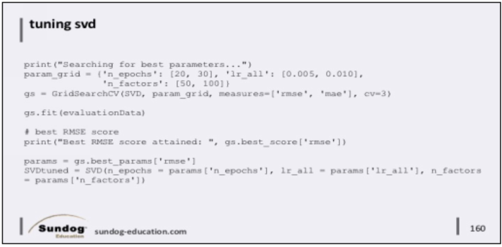
Fortunately, surpriselib contains a GridSearchCV package that helps you with hyperparameter tuning. It allows you to define a grid of different parameters you want to try out different values for, and it will automatically try out every possible combination of those parameters and tell you which ones performed the best.
Let’s look at this code snippet. If you look at the param_grid dictionary we’re setting up, you’ll see it maps parameter names to lists of values we want to try. Remember we have to run the algorithm for every possible
combination, so you don’t want to try too many values at once. We then set up a GridSearchCV with the algorithm we want to test, the dictionary of parameters we want to try out, how we’re going to measure success (in this case, by both RMSE and MAE,) and how many folds of cross-validation we want to run each time.
Then we run “fit” on the GridSearchCV with our training data, and it does the rest to find the combination of parameters that work best with that particular set of training data. When it’s done, the best RMSE and MAE scores will be in the best_score member of the GridSearchCV, and the actual parameters that won will be in the best_params dictionary. You can look up the best_params for whatever accuracy metric you want to focus on; RMSE or MAE.
So, then we can create a new SVD model using the best parameters and do more interesting things with it.
Coding Exercise
You can probably guess what your next exercise is… go ahead and try this out! Modify the SVDBakeOff script such that it searches for the best hyperparameters to use with SVD. Then, generate top-N recommendations with it and see how they look.
Oh, and if you noticed the SVDTuning.py file included in the course materials – yeah, that’s the solution to this exercise. Resist the temptation to look at it unless you really get stuck. We’ll review that file when we come back.
So we can briefly take a look at our SVDTuning.py file here to see how I went about doing hyperparameter tuning on SVD. You’ll see it’s mainly the same code we covered in the slides to set up the GridSearchCV object and use it to find the best parameters to set on SVD.
We then set up a little bake-off between SVD using the default parameters, and the tuned parameters we learned from GridSearchCV
.
Here we see the results. I settled on 20 epochs, a learning rate of 0.005, and 50 factors. You may have gotten even better results depending on how persistent you were on iterating upon the ideal numbers instead of just estimating them, as I did.
But, we can see we did indeed get a better RMSE score with these tuned results. The difference is small, but it did result in very different top-N recommendation results, which is interesting. I would consider both of these results good, but they are completely different! For example, Lord of the Rings doesn’t turn up at all when using the default parameters of SVD, but all three movies of the trilogy bubbled up when we tuned it. While the algorithm is probably correct in predicting that user number 85 would love all three of these movies, this is a good example of where results aren’t diverse enough. Often, high diversity is a sign of random recommendations that aren’t very good – but diversity that’s too low can also be a bad thing. It would be better to only recommend the first movie in the series in a case like this, and free up those other two slots for different titles. Sometimes simple little rules like that – don’t recommend more than one movie in the same series – can make a difference.