1 Introduction
This chapter is aimed at introducing and explaining some basic concepts of statistics and probability in order to aid the reader in understanding some of the more advanced concepts presented in the main text of the book. The main topics that are discussed are set theory, permutations and combinations, discrete and continuous probability distributions, descriptive statistics, and bivariate distributions.
While the main aim of this book is largely beyond the scope of these ideas, they form the basis on which the advanced techniques presented have been developed. A solid grasp of these fundamentals, therefore, is crucial to understanding the insights that can be provided by more complex techniques.
However, in explaining these ideas, the chapter briefly sketches out the core principles on which they are based. For a more comprehensive discussion, see Complete Business Statistics by Aczel and Sounderpandian (McGraw-Hill, 2009).
2 Foundations of Probability
2.1 Axioms and Set Theory
In order to understand the mathematical study of probability, it is important to first define some axioms of the field and introduce some basic set theory.
A set is a collection of objects. For example, the set of all single-digit whole numbers is {1,2,3,..,9}; the set of single-digit even numbers would be {2,4,6,8}, while the set of single-digit prime numbers would be {2,3,5,7}. A subset is a set of elements that is wholly included in some other set. So the set of all odd numbered single-digit primes {3,5,7} is a subset of the set of single-digit primes.
We can also use some basic notation to denote operations performed on two or more sets. Let us define the set of single-digit even numbers as A: {2,4,6,8}, and the set of single-digit prime numbers as B: {2,3,5,7}. A union of the two sets would include all elements of both sets, denoted by the symbol ∪. So A∪B would be {2,3,4,5,6,7,8}. An intersection of the two sets would include only the objects, or elements, present in both sets, denoted by the symbol ∩. Thus, A∩B would be {2}. A complement to a subset (usually denoted with the symbol ′) is a subset that contains all elements not present in the original subset. So A′, the complement to A, would be {1,3,5,7,9}. (It is important to point out that the complementation operation requires the definition of the full set or universal set; in this case, we assumed the set of single-digit whole numbers is the universal set.) It is possible to use these operations to include more sets—for example, we could denote the intersection of four sets called W, X, Y, and Z by writing W∩X∩Y∩Z.
In the study of probability, we can use set theory to define the possible outcomes of an experiment. We call the set of all possible outcomes of some experiment the “sample space” of that experiment. The sample space of rolling a die, for example, would be {1,2,3,4,5,6}. An event is the set of outcomes (a subset of the sample space) for which the desired outcome occurs. Thus, the event “roll an even number” would be described by the subset {2,4,6}. The event “roll an odd number” would be described by the subset {1,3,5}. The intersection of these two sets does not contain any elements. We call such sets “disjoint.” The union of these two sets describes the sample space. We call such sets a “partition” of the sample space (they are said to be mutually exclusive and collectively exhaustive).
If we have a subset A that contains our outcomes, we denote the probability of that event as P(A). To denote the probability of event A occurring given that event B has occurred, we write P(A|B). If A and B are disjoint, P(A| B) = 0. If A and B are independent events, which means that the likelihood of one occurring does not affect the likelihood of the other, then P(A| B) = P(A) and P(B| A) = P(B). From this we can see that two events can only be both disjoint and independent if one of the events has a probability of 0. What is probability of a set exactly? In the simple world of frequencies, it is relative count of the event defined by the set. For example, how often will we see the number 1 while rolling a dice? If dice were fair one would say 1/6—on average once in every six tosses.
The aim of studying probability is to understand how likely an event is to occur. Given some number of observations of an experiment (such as drawing a card from a pack), probability can tell us how likely some outcome of that experiment is (such as drawing a king, or a diamond). Set theory enables us to study these questions by supplying us with a mathematical vocabulary with which we can ask these questions.
- 1.The probability of any event occurring must be between zero and one.

- 2.Every experiment must result in an event. The probability of nothing (denoted as null or ∅) happening is zero. The probability of sample space (denoted here by S—but is not a standard notation for something) happening is one.
![$$ \begin{array}{c}\displaystyle\mathrm{P}\left(\varnothing \right)=0\\[6pt] \mathrm{P}\left(\mathrm{S}\right)=1 \end{array} $$](../images/428412_1_En_30_Chapter/428412_1_En_30_Chapter_TeX_Equb.png)
- 3.If two or more events are mutually exclusive (the subsets that describe their outcomes are disjoint), then the probability of one of them happening is simply the sum of the individual probabilities.

2.2 Bayes’ Theorem
Bayes’ theorem is one of the most powerful tools in probability. The theorem allows us to relate conditional probabilities, or the likelihood of an event occurring given that some other event has occurred, to each other.


But A∩B and B∩A are the same!
Therefore, Bayes’ theorem of conditional probability provides the foundation for one of the most important machine learning algorithms—the naïve machine learning algorithm. The algorithm postulates the likelihood of an event occurring (the prior), absorbs and analyzes new data (the likelihood), and then updates its analysis to reflect its new understanding (the posterior).
We can use Bayes’ theorem to analyze a dataset in order to understand the likelihood of certain events given other events—for example, the likelihood of owning a car given a person’s age and yearly salary. As more data is introduced into the dataset, we can better compute the likelihood of certain characteristics occurring in conjunction with the event, and thus better predict whether a person with a random set of characteristics may own a car. For example, say 5% of the population is known to own a car—call this A. This can be inferred from your sample data. In your sample, 12% are between 30 and 40 years of age—call this B. In the subset of persons that own a car, 25% are between age 30 and 40—this is (B| A). Thus, P(A) = 0.05. P(B) = 0.12. P(B| A) = 0.25. Thus,  . In other words, 60% of those that are between 30 and 40 years of age own a car.
2.3 Random Variables and Density Functions
Until now we have discussed probability in terms of sample spaces, in which the likelihood of any single outcome is the same. We will now consider experiments in which the likelihood of some outcomes is different than others. These experiments are called random variables. A random variable assigns a numerical value to each possible outcome of an experiment. These variables can be of two types: discrete or continuous.
Discrete random variables are experiments in which there are a finite number of outcomes. We might ask, for example, how many songs are on an album. Continuous random variables, on the other hand, are experiments that might result in all possible values in some range. For example, we might model the mileage driven of a car as a continuous random variable.
Normally, we denote an experiment with a capital letter, such as X, and the possibility of an outcome with a small letter, such as x. Therefore, in order to find out the likelihood of X taking the value x (also known as x occurring), we would write P(X = x). From the axioms of probability, we know that the sum of all P(x) must be 1. From this property, we can construct a probability mass function (PMF) P for X that describes the likelihood of each event x occurring.
Probability from rolling a fair die
Outcome (x) | Probability (p) | PMF: P(X = x) = p |
|---|---|---|
1 | 1/6 | P(X = 1) = 1/6 |
2 | 1/6 | P(X = 2) = 1/6 |
3 | 1/6 | P(X = 3) = 1/6 |
4 | 1/6 | P(X = 4) = 1/6 |
5 | 1/6 | P(X = 5) = 1/6 |
6 | 1/6 | P(X = 6) = 1/6 |
The PMF for each outcome P(X = x) (x = 1,2,…,6) is equal to 1/6.
Probability from rolling an altered die
Outcome (x) | Probability (p) | PMF: P(X = x) = p |
|---|---|---|
1 | 1/12 | P(X = 1) = 1/12 |
2 | 3/12 | P(X = 2) = 1/6 |
3 | 1/6 | P(X = 3) = 1/6 |
4 | 1/6 | P(X = 4) = 1/6 |
5 | 3/12 | P(X = 5) = 1/4 |
6 | 1/12 | P(X = 6) = 1/6 |
In this case, the PMF tells us that the likelihood for some outcomes is greater than the likelihood for other outcomes. The sum of all the PMFs is still equal to one, but we can see that the die is no longer equally likely to produce each outcome.
A second useful function is the cumulative distribution function (CDF), which is defined as P(X ≤ x). When x is at its greatest, the CDF is equal to one. For the fair die, P(X ≤ 5) = 5/6. For the unfair die,  .
.
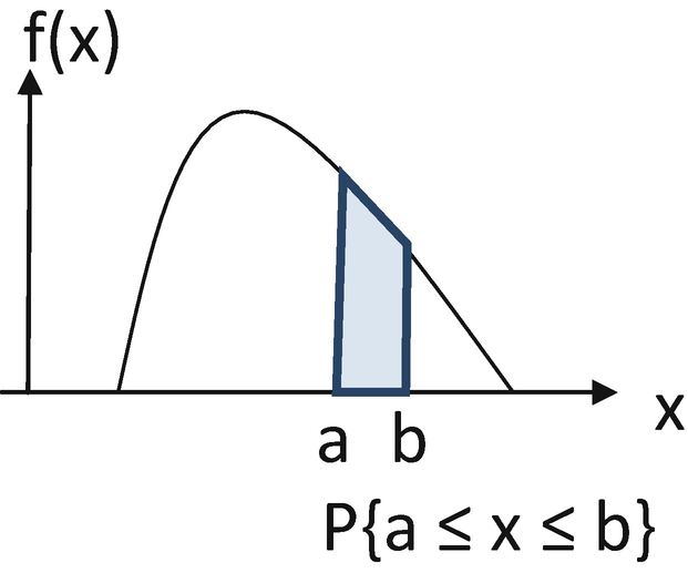
Computing probability of x between a and b
More generally, P(a ≤ X ≤ b) = P(X ≤ b) − P(X ≤ a). In this figure, the function f(x) measures the height at every point of the curve. Therefore, f is called the probability density function or the density function.
- (a)
f(x) ≥ 0 for every x.
- (b)
 . (In general, this integral need extend only over the range over which f is defined. This range is also called the support of the probability distribution.)
2.4 Mean and Variance
However, describing the probability density function of a random variable is often cumbersome. As random variables can take any number of possible values, visualizing a function can be difficult. In order to make such a process simpler, we use two main tools of summarization: the mean and the variance. The mean is a measure of central tendency—the expected or average value of the distribution. The variance is a measure of dispersion—how clustered together the outcomes are. These two measures can give us an idea of the distribution and its relation to the experiment.
The mean of a random variable is also called its expected value—the probability weighted average that we “expect” will occur. It is calculated as the sum of the products of each outcome x and the likelihood of that outcome P(X = x), and is denoted by μ. (In general, the value of a function, say G(x), computed using the PDF f, is written as ![$$ \mathrm{E}\left[\mathrm{G}\right]={\int}_{-\infty}^{+\infty }G(x)f(x) dx $$](../images/428412_1_En_30_Chapter/428412_1_En_30_Chapter_TeX_IEq4.png) . This is called the expected value of G under f. Thus, E[X] is the expected value of X, which is also referred to as mean.)
. This is called the expected value of G under f. Thus, E[X] is the expected value of X, which is also referred to as mean.)

![$$ \mathrm{E}\left[\mathrm{X}\right]=\underset{-\infty }{\overset{+\infty }{\int }} xf(x) dx $$](../images/428412_1_En_30_Chapter/428412_1_En_30_Chapter_TeX_Equh.png)

This tells us that the “expected” value of an experiment may not actually be equal to a value that the experiment can take. We cannot actually ever roll 3.5 on a die, but we can expect that on average, the value that any die will take is 3.5.
In the case of a continuous random variable, the mean of the PDF cannot be computed using discrete arithmetic. However, we can use calculus to derive the same result.

Here, the limits of the integral are assumed to be the range over which f is defined—and omitted in the sequel below.
The second important summary is the variance. The variance of an experiment is a measure of how far away on average any outcome is from the mean. Knowing the variance of a function allows us to understand how spread out the outcomes are relative to the mean. In order to find this, we can measure the distance between each outcome and the mean: (x − μ), and add them. By definition, however, some values are below the mean, while other values are above the mean. Simply summing the distances of these outcomes from the mean will lead us to cancel out some outcomes. In order to circumvent this, we add the squares of the distances: (x − μ)2.


![$$ Var(X)=\int {\left[x-E(X)\right]}^2.f(x) dx=\int {\left[x-\mu \right]}^2.f(x) dx $$](../images/428412_1_En_30_Chapter/428412_1_En_30_Chapter_TeX_Equm.png)
As variance is measured in terms of the square of the random variable, it is not measured in the same units as the distribution itself. In order to measure dispersion in the same units as the distribution, we can use the standard deviation (denoted as σ), which is the square root of the variance.
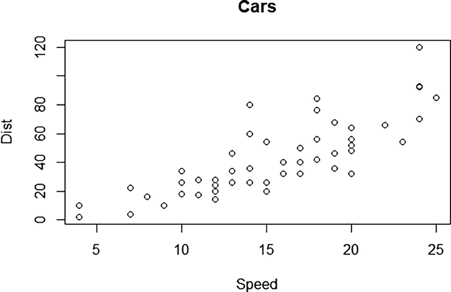
Scatter plot—distribution of cars dataset
2.5 Bernoulli Distribution
The Bernoulli distribution is a type of discrete random variable which models an experiment in which one of two outcomes can occur. For example, a question with a yes/no answer or a flip of a coin can be modeled using Bernoulli distributions.
As there are only two outcomes (say x 1 and x 2), knowing the likelihood of one outcome means that we know the likelihood of the other outcome, that is, if P(X = x1) = p, then P(X = x2) = 1 − p. This is denoted by X ∼ Bernoulli (p). The symbol ∼ stands for “distributed as.”
A fair coin will have P(X = heads) = 0.5. An unfair coin may have P(X = heads) = 0.45, which would mean P(X = tails) = 0.55.
But what if we have repeated trials? Say, many Bernoulli trials? See further.
2.6 Permutations and Combinations
In this case, we can use combinatorics to identify how many ways there are of picking combinations. Combinatorics deals with the combinations of objects that belong to a finite set. A permutation is specific ordering of a set of events. For example, the coin flipping heads on the first, third, and fourth flip out of five flips is a permutation: HTHHT. Given “n” objects or events, there are n! (n factorial) permutations of those events. In this case, given five events: H, H, H, T, and T, there are 5! ways to order them. 5! = 5*4*3*2*1 = 120. (There may be some confusion here. Notice that some of these permutations are the same. The 120 number comes up because we are treating the three heads as different heads and two tails as different tails. In one other way of saying this, the five events are each different—we would have been better if we had labeled the events 1,2,3,4,5.)
However, sometimes we may want to choose a smaller number of events. Given five events, we may want a set of three outcomes. In this case, the number of permutations is given by 5!/(5 − 3)! = 5*4*3 = 60. That is, if we have “n” events, and we would like to choose “k” of those events, the number of permutations is n!/(n − k)! If we had five cards numbered 1–5, the number of ways that we could choose three cards from them would be 60. (In another way of seeing this, we can choose the first event in five ways, the second in four ways, and the third in three ways, and thus 5 * 4 * 3 = 60.)
A combination is the number of ways in which a set of outcomes can be drawn, irrespective of the order in which the outcomes are drawn. If the number of permutations of k events out of a set of n events is n!/(n − k)!, the number of combinations of those events is the number of permutations, divided by the number of ways in which those permutations occur: n!/((n − k)!k!). (Having drawn k items, they themselves can be permuted k! times. Having drawn three items, we can permute the three 3! times. The number of combinations of drawing three items out of five equals 5!/((5 − 3)!3!) = 60/6 = 10.)
Using the theory of combinations, we can understand the binomial distribution.
2.7 Binomial Distribution

Consider, however, the probability of four out of the ten flips being heads. There are many orders (arrangements or sequences) in which the four flips could occur, which means that the likelihood of P(X = 4) is much greater than 0.0011351. In this case, it is given by: 10!/[(10 − 4)!*4!]*(0.45)4*(0.55)6 = 0.238 (= 210*0. 0.0011351, where 210 represents the number of combinations of drawing four out of ten items.)
![$$ \mathrm{P}\left(\mathrm{X}=\mathrm{x}\right)=\mathrm{n}!/\left[\left(\mathrm{n}-\mathrm{x}\right)!\mathrm{x}!\right]\ast {\mathrm{p}}^{\mathrm{x}} * {\left(1-\mathrm{p}\right)}^{\mathrm{n}-\mathrm{x}} $$](../images/428412_1_En_30_Chapter/428412_1_En_30_Chapter_TeX_Equo.png)
Binomial distribution with n = 10 and p = 0.25
X | P |
|---|---|
1 | 0.187712 |
2 | 0.281568 |
3 | 0.250282 |
4 | 0.145998 |
5 | 0.058399 |
6 | 0.016222 |
7 | 0.003090 |
8 | 0.000386 |
9 | 0.000029 |
10 | 0.000001 |
2.8 Poisson Distribution
The Poisson distribution is an extension of the binomial distribution for situations in which the number of trials is very large, the likelihood of an event occurring is very small, and the mean (n*p) of the distribution is finite.
![$$ \mathrm{P}\left(\mathrm{X}=\mathrm{x}\right)=\frac{\left[{e}^{-\mathrm{n}\ast \mathrm{p}}.{\left(\mathrm{n}\ast \mathrm{p}\right)}^x\right]}{x!} $$](../images/428412_1_En_30_Chapter/428412_1_En_30_Chapter_TeX_Equp.png)
We use λ to denote nxp, the mean, We write this as X ∼ Poisson(λ).
Poisson distribution with mean = 2.5
X | P |
|---|---|
1 | 0.205212 |
2 | 0.256516 |
3 | 0.213763 |
4 | 0.133602 |
5 | 0.066801 |
6 | 0.027834 |
7 | 0.009941 |
8 | 0.003106 |
9 | 0.000863 |
10 | 0.000216 |
2.9 Normal Distribution
The normal distribution is one of the most important continuous distributions, and can be used to model a number of real-life phenomena. It is visually represented by a bell curve.
Just as the binomial distribution is defined by two parameters (n and p), the normal distribution can also be defined in terms of two parameters: μ (mean) and sigma (standard deviation). Given the mean and standard deviation (or variance) of the distribution, we can find the shape of the curve. We can denote this by writing X ∼ N(μ, sigma).
- 1.
The mean, median, and mode are equal.
- 2.
The curve is symmetric about the mean.
- 3.
The total area beneath the curve is equal to one.
- 4.
The curve never touches the x-axis.
The mean of the normal distribution represents the location of centrality, about which the curve is symmetric. The standard deviation specifies the width of the curve.
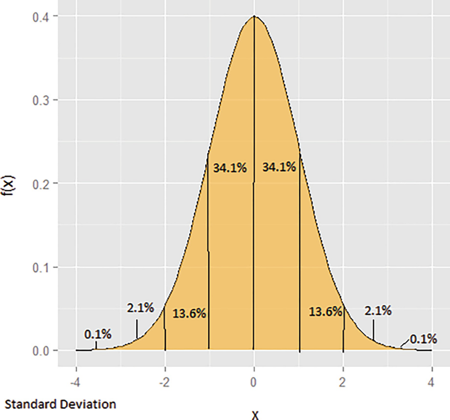
Shape of the normal distribution
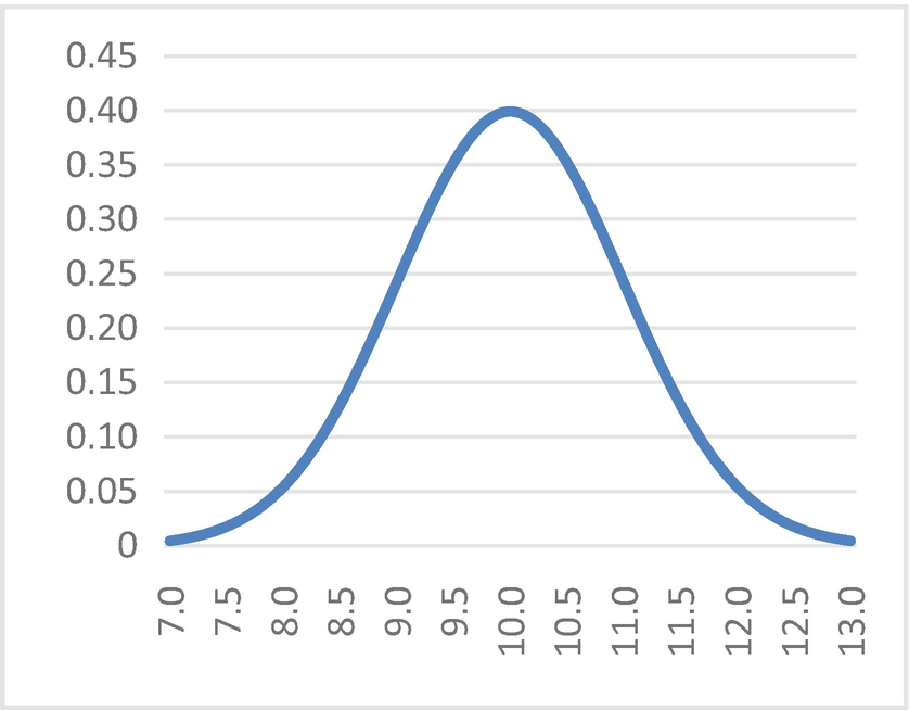
Normal distribution with mean = 10 and standard deviation = 1
However, computing the normal distribution can become difficult. We can use the properties of the normal distribution to simplify this process. In order to do this, we can define the “standard” normal distribution, denoted Z, as a distribution that has mean 0 and standard deviation 1. For any variable X described by a normal distribution, z = (X − μ)/sigma. The z-score of a point on the normal distribution denotes how many standard deviations away it is from the mean. Moreover, the area beneath any points on a normal distribution is equal to the area beneath their corresponding z-scores. This means that we only need to compute areas for z-scores in order to find the areas beneath any other normal curve.
- 1.
P(Z > z) = 1 − p(Z < z)
- 2.
P(Z < − z) = P(Z > z)
- 3.
P(z1 < Z < z2) = P(Z < z2) − P(Z < z1)
Standard normal distribution tables provide cumulative values for P(Z < z) until z = 0.5. Using symmetry, we can derive any area beneath the curve from these tables.
The normal distribution is of utmost importance due to the property that the mean of a random sample is approximately normally distributed with mean equal to the mean of the population and standard deviation equal to the standard deviation of the population divided by the square root of the sample size. This is called the central limit theorem. This theorem plays a big role in the theory of sampling.
3 Statistical Analysis
Merriam-Webster defines statistics as a “branch of mathematics dealing with the collection, analysis, interpretation, and presentation of masses of numerical data.”1 Statistics, therefore, is concerned with recording occurrences that take place, and attempting to understand why those occurrences do so in that manner. A statistic, however, is also a “quantity (such as the mean of a sample) that is computed from a sample.” Thus, we may have several statistics, or facts, about a set of data that we have gathered, which we have found through the use of statistics.
A “dataset” is simply a recording of all the pieces of information we have collected. If we were examining cars, our dataset might include each car’s color, age, model, place of manufacture, and so on.
A “population” is the sum total of all pieces of data in the field we are examining. For example, if we wanted to investigate the mileage of every car in the world, our population would consist of each and every car that has ever been made.
A “sample” is a subset of the population, which we have actually recorded. Often statistics must rely on samples as it is infeasible to record the entire population—finding the mileage of every car ever made sounds like an impossible task.
The difference between a sample and a population is key to statistical analysis. If we use a dataset that consists of the entire population of cars in the world (imagining for a moment that we have been able to collect it) we can know for sure that we have accounted for every possible recording that is available. However, if we are using a sample that we have drawn from the population, we cannot know for sure that there are other findings that we have missed that may drastically change the nature of our dataset. Refer Chap. 2 for more details.
This is important because collection is only one part of statistics. After collecting data, we must analyze it in order to find insights about the dataset we have obtained, and thus about the world that we have recorded in our dataset. These tools of analysis, despite being very simple, can be incredibly profound and inform the most advanced computational tools.
The use of data analysis that helps to describe, show, or summarize data in a way that helps us identify patterns in the dataset is known as descriptive statistics. The tools we use to make predictions or inferences about a population are called inferential statistics. There are two main types of statistical analysis. The first is univariate analysis, which describes a dataset that only records one variable. It is mainly used to describe various characteristics of the dataset. The second is multivariate analysis, which examines more than one variable at the same time in order to determine the empirical relationship between them. Bivariate analysis is a special case of multivariate analysis in which two variables are examined.
In order to analyze a dataset, we must first summarize the data, and then use the data to make inferences.
The first type of statistic that we can derive from a variable in a numerical dataset is measures of “central tendency,” or the tendency of data to cluster around some value. The arithmetic mean, or the average, is the sum of all the values that the variable takes in the set, divided by the number of values in the dataset. This mean corresponds to the expected value we find in many probability distributions.
The median is the value in the dataset above which 50% of the data falls. It partitions the dataset into two equal halves. Similarly, we can divide the data into four equal quarters, called quartiles, or 100 equal partitions, called percentiles.
If there is a value in the dataset that occurs more times (more often) than any other, it is called the mode.

![$$ r- th\ central\ moment={\mu}_r=\frac{\sum {\left( Data\ value- Mean\right)}^r}{n}=E\left[{\left(X-\mu \right)}^r\right]. $$](../images/428412_1_En_30_Chapter/428412_1_En_30_Chapter_TeX_Equr.png)

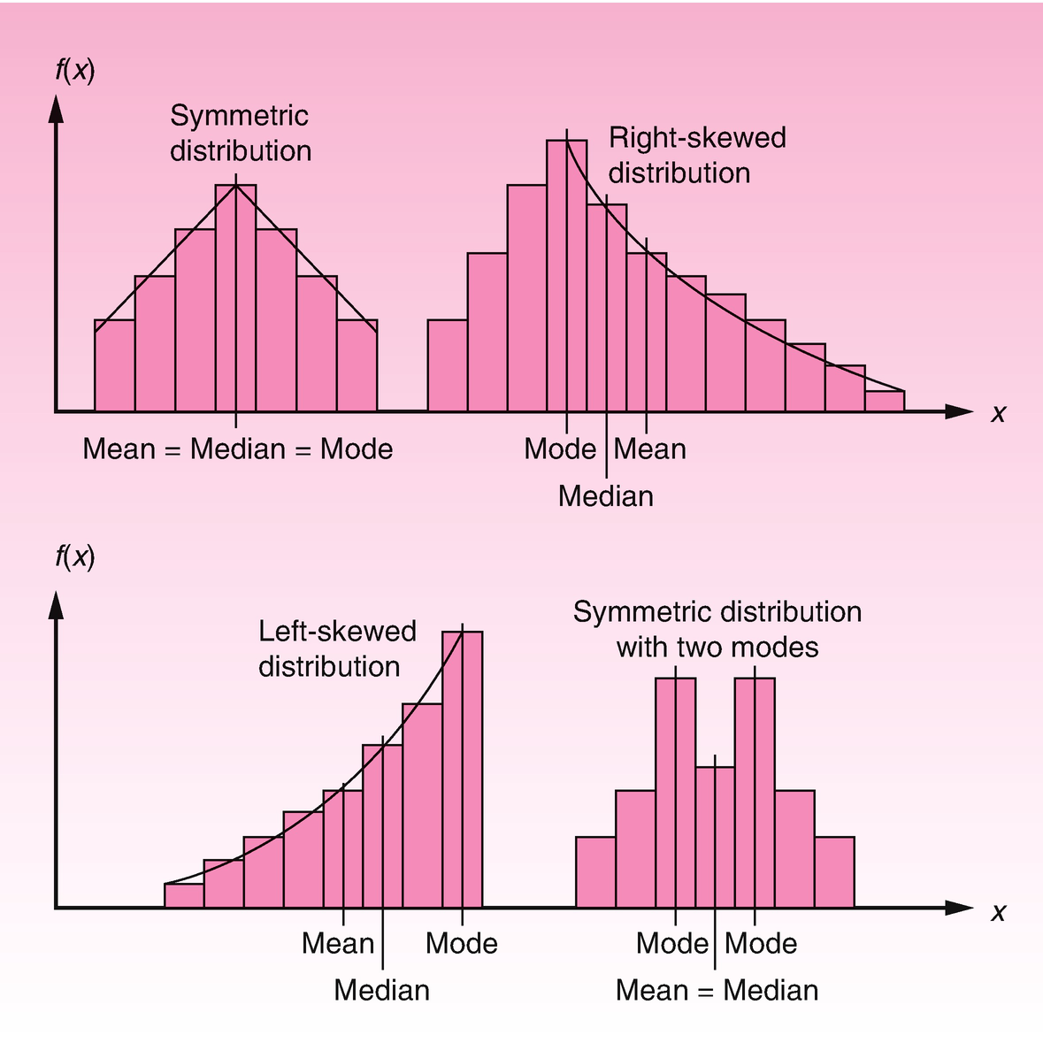
Different types of distributions

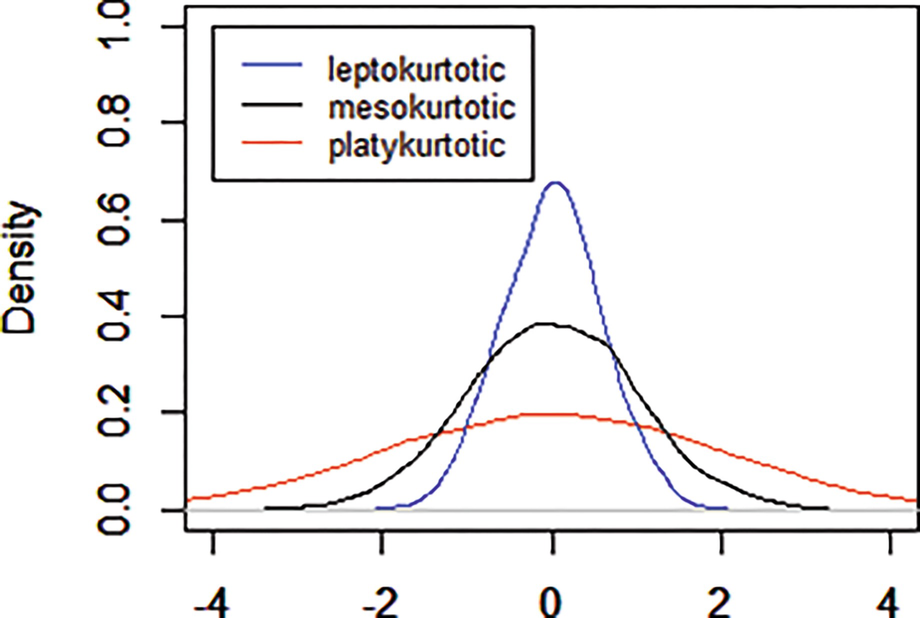
Normal distributions with different kurtosis. The red line represents a frequency curve of a long tailed distribution. The blue line represents a frequency curve of a short tailed distribution. The black line is the standard bell curve
4 Visualizing Data
Frequency distribution table
Color | Frequency |
|---|---|
Red | 10 |
Green | 14 |
Black | 12 |
White | 19 |
Blue | 11 |
Orange | 2 |
Purple | 1 |
Graphs and charts can also be an effective tool to portray characteristics of data. In a pie chart, a circle is divided into various “pies” that denote the ratio of the dataset’s composition. In a bar graph, the size of the variable for several categories is portrayed as a vertical bar. In a scatter plot, datapoints that consist of two values are plotted on a two-dimensional graph that can portray a relationship between the two variables.
Using bar graphs to represent datasets can become visually confusing. In order to avoid this, we can use box plots, which simplify the datasets by dividing them into partitions of equal size. Then, by drawing a box plot, we can understand intuitively whether the dataset is skewed and how the data is concentrated.
- 1.
Divide the data into quartiles
- 2.
On an axis representing the variable, draw a box of length equal to Q3-Q1
- 3.
From each side of the box, extend a line to the maximum and minimum values
- 4.
Indicate the median in the box with a solid line
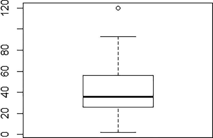
Box plot of distance variable in cars dataset
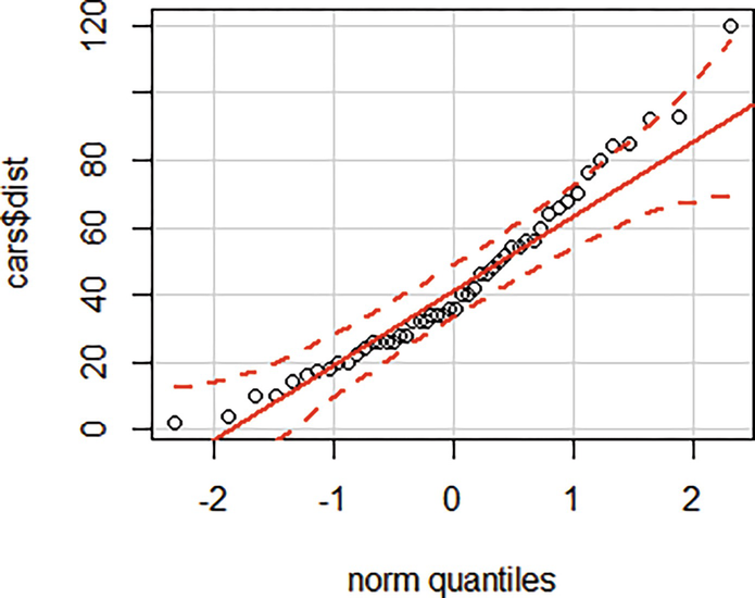
Q-Q plot of distance variable in cars dataset
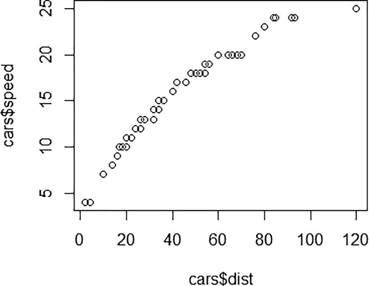
Q-Q plot of distance versus speed variable in cars dataset
5 Bivariate Analysis
Bivariate analysis is among the most basic types of analysis. By using the tools developed to consider any single variable, we can find correlations between two variables. Scatter plots, frequency tables, and box plots are frequently used in bivariate analysis.
![$$ \mathrm{Cov}\left(\mathrm{X},\mathrm{Y}\right)=\mathrm{E}\left[\right(\mathrm{X}-\mathrm{E}\left(\mathrm{X}\left)\right)\left(\mathrm{Y}-\mathrm{E}\left(\mathrm{Y}\right)\right)\right]=\mathrm{E}\left(\mathrm{X}\mathrm{Y}\right)-\mathrm{E}\left(\mathrm{X}\right)\mathrm{E}\left(\mathrm{Y}\right) $$](../images/428412_1_En_30_Chapter/428412_1_En_30_Chapter_TeX_Equu.png)

The coefficient of correlation always lies between −1 and +1. As it moves from negative to positive, the variables change from moving perfectly against one another to perfectly with one another. At 0, the variables do not move with each other (to be perfectly honest we need to say in an average sense). Independent variables are uncorrelated (but uncorrelated variables are not independent with some exceptions such as when both variables are normally distributed).
- 1.
Corr(X,X) = 1 (X is perfectly correlated with itself)
- 2.
Cov(X,X) = Var(X) (The dispersion of X compared to itself is the variance)
- 3.
Var(X + Y) = Var(X) + Var(Y) + 2Cov(X,Y)
- 4.
Var(X − Y) = Var(X) + Var(Y) − 2Cov(X,Y)
It is important to note that correlation is a powerful but simple tool, which may not catch nuanced observations. For example, if X and Y are related in a quadratic manner, their correlation will be 0 even though we know that there is a relationship between the two variables. Moreover, the existence of rogue datapoints, or outliers, can change the value of correlation dramatically. Most importantly, it is critical to remember that correlation does not imply causation. Simply because two variables are correlated in some way does not give us enough evidence to infer a relationship between them. More details are given in the Chap. 7.
For the variables cars$dist and cars$speed, covariance = 109.95 and correlation = 0.8068.