Appendix B
Matrix Operations with MATLAB

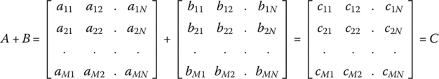
B.1 Addition and Subtraction

(B.1a)

(B.1b)

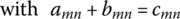
B.2 Multiplication

(B.2a)

(B.2b)

• (cf.) For this multiplication to be done, the number of columns of A must equal the number of rows of B.
• (cf.) Note that the commutative law does not hold for the matrix multiplication, i.e. AB ≠ BA.

B.3 Determinant

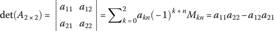
The determinant of a K × K (square) matrix A = [a_mn] is defined by

(B.3)

where the minor M_kn is the determinant of the (K−1) × (K−1) (minor) matrix formed by removing the kth row and the nth column from A and c_kn = (−1)^k+nM_kn is called the cofactor of a_kn.

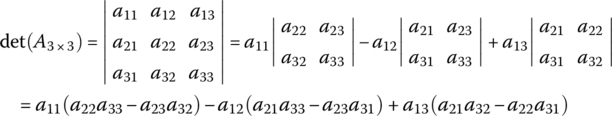
Especially, the determinants of a 2 × 2 matrix A_2×2 and a 3 × 3 matrix A_3×3 are

(B.4a)

(B.4b)

Note the following properties.

• If the determinant of a matrix is zero, the matrix is singular.
• The determinant of a matrix equals the product of the eigenvalues of a matrix.
• If A is upper/lower triangular having only zeros below/above the diagonal in each column, its determinant is the product of the diagonal elements.
• det(A^T) = det(A); det(AB) = det(A) det(B); det(A^‐1) = 1/det(A)

B.4 Inverse Matrix

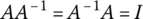
The inverse matrix of a K × K (square) matrix A = [a_mn] is denoted by A⁻¹ and defined to be a matrix which is pre‐multiplied/post‐multiplied by A to form an identity matrix i.e. satisfies

(B.5)

An element of the inverse matrix A⁻¹=[α_mn] can be computed as

(B.6)

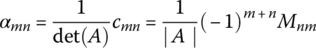
where M_nm is the minor of a_nm and c_mn = (‐1)^m+nM_nm is the cofactor of a_mn.

Note that a square matrix A is invertible/nonsingular if and only if

• no eigenvalue of A is zero or equivalently,
• the rows (and the columns) of A are linearly independent or equivalently, and
• the determinant of A is nonzero.

---

Example B.1 Matrix Inversion

Let us find the inverse of a 3 × 3 matrix

(1)

where the cofactors are

We can use Eqs. (B.3) and (B.6) to get the determinant and the inverse matrix as

(2)

(3)

---

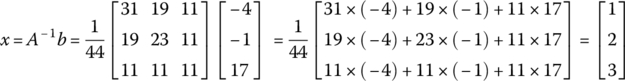
B.5 Solution of a Set of Linear Equations Using Inverse Matrix

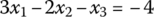
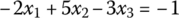
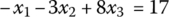
Let us consider the following set of linear equations in three unknown variables x₁, x₂, and x₃:

This can be formulated in the matrix‐vector form

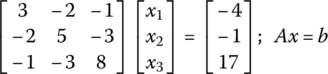
so that it can be solved as

B.6 Operations on Matrices and Vectors Using MATLAB

The following statements and their running results illustrate the powerful usage of MATLAB in dealing with matrices and vectors.

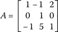
>>a= [-2 2 3] % a 1x3 matrix (row vector)
  a = -2 2 3
>>b= [-2; 2; 3] % 3x1 matrix (column vector)
  B = -2
       2
       3
>>b= a.' % transpose

>>A= [1 -1 2; 0 1 0; -1 5 1] % a 3x3 matrix

>>A(1,2) % will return -1
>>A(:,1) % will return the 1st column of the matrix A
  ans = -1
         0
        -1
>>A(:,2:3) % will return the 2nd and 3rd columns of the matrix A 
  ans = -1  2
         1  0
         5  1
>>c= a*A % vector–matrix multiplication
  C= -5 19 -1
>>A*b
  ans =  2
         2
        15
>>A*a % not permissible for matrices with incompatible dimensions
  ??? Error using ==> mtimes
  Inner matrix dimensions must agree
>>a*c' % Inner product : multiply a with the conjugate transpose of c
  ans = 45
>>a.*c % (termwise) multiplication element by element
  ans = 10 38 -3
>>a./c % (termwise) division element by element 
  ans = 0.4000  0.1053  -3.0000
>>det(A) % determinant of matrix A
  ans = 3
>>inv(A) % inverse of matrix A
  ans =  0.3333   3.6667  -0.6667
         0        1.0000   0
         0.3333  -1.3333   0.3333
>>[V,E]= eig(A) % eigenvector and eigenvalue of matrix A
   V = 0.8165            0.8165             0.9759
       0                 0                  0.1952
       0 + 0.5774i       0 - 0.5774i        0.0976
   E = 1.0000 + 1.4142i  0                  0
       0                 1.0000 - 1.4142i   0
       0                 0                  1.0000
>>I= eye(3) % a 3x3 identity matrix
>>O= zeros(size(I)) % a zero matrix of the same size as I
>>A= sym('[a b c; d e f]') % a matrix consisting of (non-numeric) symbols
  A =   [ a, b, c]
        [ d, e, f]
>>B= [1 0; 0 1; 1 1]
  B =   1   0
        0   1
        1   1
>>A*B
  ans = [a+c, b+c]
        [d+f, e+f]