A simple recommender system

Here is an item-to-item version in which the utility matrix is Boolean: .

Recommender algorithm 1 is as follows. Given an input list of (i, j) pairs, representing purchases of items y_j bought by users x_i:

1. Initialize the utility matrix (u_ij) with m rows and n columns, where m is the number of users and n is the number of items.
2. For each pair (i, j) in the input list, set u_ij = 1.
3. Initialize the similarity matrix (s_jk) with n rows and n columns.
4. For each j = 1…n and each k = 1…n, set s_jk = s(u, v), the cosine similarity of the j^th column u and the k^th column v of the utility matrix.
5. For a given user-purchase pair (i, j) (that is, u_ij = 1):
   • Find the set S of items not bought by user i
   • Sort the items in S according to how similar they are to item j
6. Recommend the top n₁ elements of S, where n₁ is a specified constant much less than n.

To implement this algorithm, we need an input list of purchases. The program in Listing 9.2 generates a random list of pairs, where the pair (i, j) represents the purchase of item j by user i:

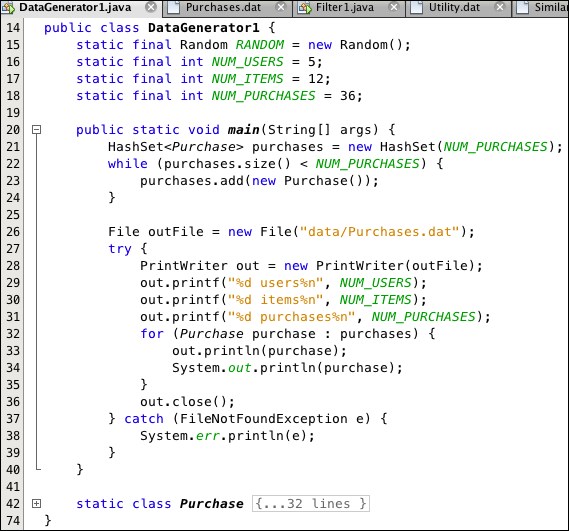
Listing 9.2: Program to generate user-item pairs

The program generates 36 (i, j) pairs, where 1 ≤ i ≤ 5 and 1 ≤ j ≤ 12, representing 36 purchases with 5 users and 12 items. These are stored in the external file Purchases1.dat, shown in Figure 9.2:

Figure 9.2: Purchases file

It also inserts three header lines specifying the numbers of users, items, and purchases.

The static nested Purchase class (lines 42-73) is shown in Listing 9.3:

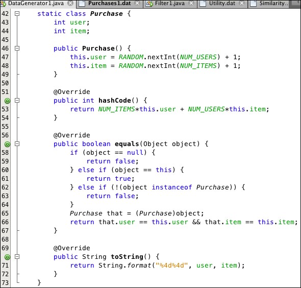
Listing 9.3: The Purchase class in the DataGenerator1 program

The random values for the user and item numbers are generated in the default constructor at lines 47 and 48. The hashCode() and equals() methods are included in case the objects are to be used in a Set or Map collection.

The Filter1 program in Listing 9.4 implements steps 1-4 of the algorithm, filtering the Purchases1.dat file to generate the Utility1.dat and Similarity1.dat files to store the utility and similarity matrices. Its methods for computing and storing the matrices are shown in Listing 9.5 and Listing 9.6. The utility matrix entries are read directly from the Purchases1.dat file. The similarity matrix entries are computed by the cosine() method, shown with its auxiliary dot() and norm() methods in Listing 9.7. The resulting Utility1.dat and Similarity1.dat files are shown in Figure 9.3 and Figure 9.4.

The code at lines 90-91 in Listing 9.7 prevents division by zero. If the value of denominator is zero, then either the j^th column or the k^th column of the utility matrix is the zero vector; that is, all its components are zero. In that case, the cosine similarity will be 0.0, by default.

Steps 5 and 6 of the recommender algorithm 1 are implemented by the Recommender1 program in Listing 9.8. Its methods are shown separately in Listing 9.9 through Listing 9.12. Two sample runs of the program are shown in Figure 9.5 and Figure 9.6:

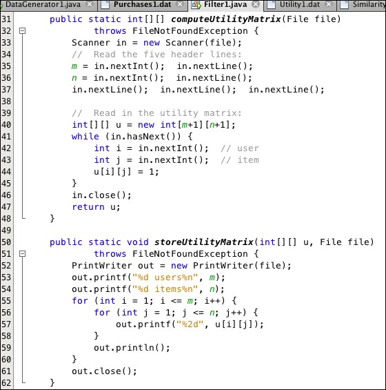
Listing 9.4: Program to filter the purchases list

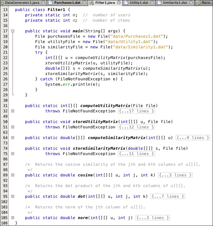
Listing 9.5: Compute and store the utility matrix

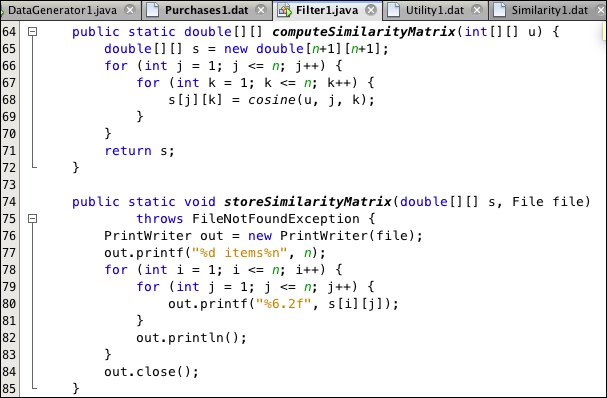
Listing 9.6: Compute and store the similarity matrix

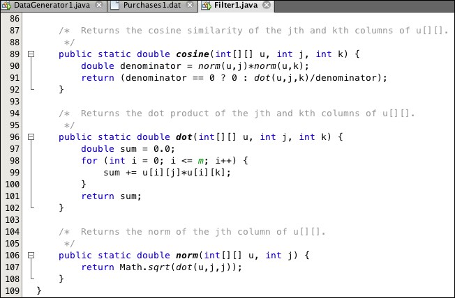
Listing 9.7: Methods for computing similarity

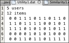
Figure 9.3: The Utility.dat file

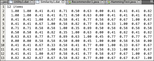
Figure 9.4: The Similarity.dat file

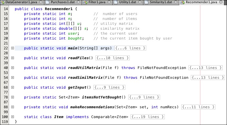
Listing 9.8: The Recommender1 program

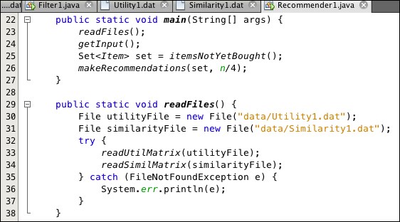
Listing 9.9: Methods for the Recommender1 program

Step 5 of the algorithm is implemented by the method called at line 25, and step 6 is implemented by the makeRecommendations() method called at line 26. Note that we have chosen the value n/4 for n₁.

The getInput() method (Listing 9.11) interactively reads a user number and item number, representing a new purchase. Then the itemsNotYetBought() method returns a set of Item objects that have not yet been bought by that user. Since we are using the TreeSet<Item> class, the set remains sorted after each addition (at line 82). The ordering is done in accordance with the overridden compareTo() method defined at lines 107-112 in Listing 9.12. When two items are compared, the one whose similarity to the bought item is greater will precede the other. This implements step 5, the second part of the algorithm. Consequently, when the set is passed to the makeRecommendation() method at line 26, its elements are already ordered in decreasing similarity to the bought item.

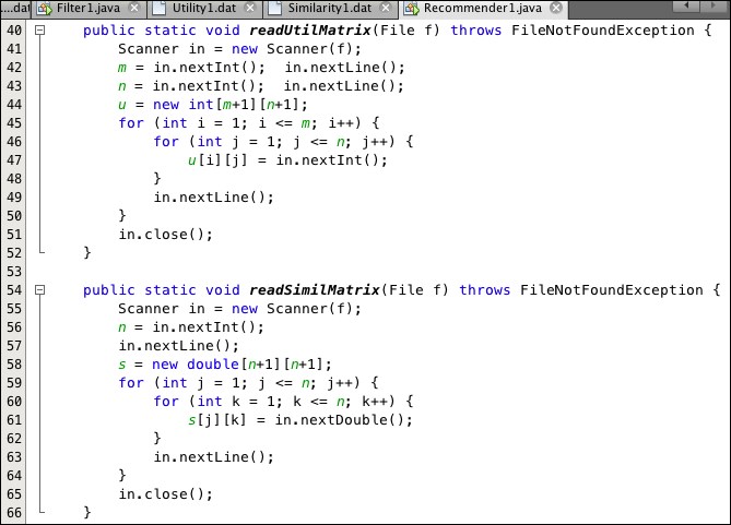
Listing 9.10: File reading methods for Recommender1 program

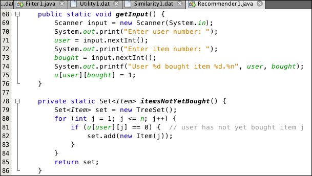
Listing 9.11: Methods for Recommender1 program

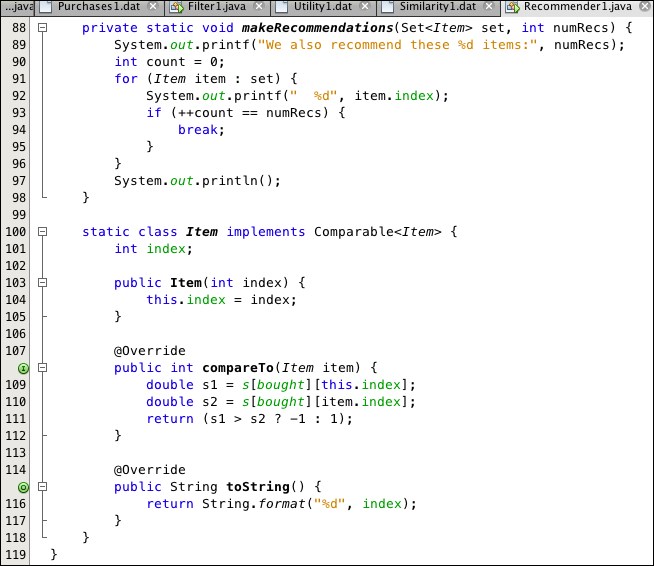
Listing 9.12: Nested Item class for Recommender1 program

The nested Item class implements the Comparable<Item> interface, which is necessary for using the Set<Item> interface. That, in turn, requires the overriding of the compareTo(Item) method (at lines 107-112). Lines 109-110 define s1 and s2 to be the similarity values (from the similarity matrix) of the implicit argument (this) and the explicit argument (item) to the bought item. If s1 > s2, meaning that this is more similar than item is to the bought item, then the method returns -1, which means that this should precede item in the set's ordering. That keeps the elements that are more similar to the bought item in front of the others. Consequently, when the for-each loop at lines 91-96 iterates through the first numRecs of the set, those elements get recommended.

The first sample run of the Recommender1 program is shown in Figure 9.5:

Figure 9.5: Run 1 of the Recommender1 program

The interactive input tells the program that user #1 has bought item #1. The utility matrix (Figure 9.3) shows that, other than item #1, item #2, item #6, item #9, and item #12 have not yet been bought by user #1. Thus, the set defined at line 25 is {2, 6, 9, 12}. But the set is ordered according to the similarity matrix (Figure 9.4), which shows that the similarities of those four items are 1.00, 0.50, 0.41, and 0.82 in the first row (corresponding to bought item #1). Thus, as an ordered set, it is (2, 12, 6, 9). The value of n/4 is 12/4 = 3, so the makeRecommendations() method at line 26 prints the first three items of that ordered set: 2, 12, and 6.

The second sample run of the program is shown in Figure 9.6:

Figure 9.6: Run 2 of the Recommender1 program

This time, user #2 has bought item #3. The other items that user #2 has not yet bought are item #8, item #9, and item #11. Their similarities to the bought item #3 are 0.58, 0.67, and 1.00, respectively, so the ordered set is (11, 9, 8). Those three are then recommended.

In the first run, the similarity of item #2 to item #1 was found to be 1.00 (that is, 100 percent). That fact can be seen directly from the utility matrix: column #2 and column #1 are identical – they're both (0, 1, 1, 0, 0). In the second run, item #3 and item #11 have 100 percent similarity: both columns are (1, 0, 1, 0, 1). In both runs, the first recommendation is an item that was uniformly rated the same as the one that the user has just bought.