3.1 Evolutionary Computation
Evolutionary Computation (EC) is a branch of Computational Intelligence (CI) and a subfield of Artificial Intelligence (AI). EC is a family of algorithms/techniques inspired by the principles of biological evolution. The origins of EC can date back to the late 1950s, when the earliest EC paradigms were proposed [15, 48]. With the development of several decades, EC becomes a hot research area with significant attention received over the world. EC techniques have been successfully applied to many real-world optimisation and learning problems [15].
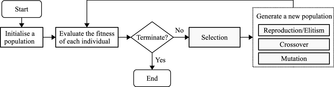
EC techniques are known as population-based search or optimisation techniques. The key idea of EC techniques is to search for the best solution to a problem using a population of individuals via an iterative process, where every individual represents a solution to the problem. In EC techniques, a fitness function is employed to evaluate the goodness of the individuals and guide the search towards better areas. A each iteration/generation, a population of new individuals are generated to replace the current population according to different operations. The search/optimisation process stops when a termination criterion is satisfied. If the evolutionary process is terminated, the best solution is returned. The main process of EC techniques is outlined in Fig. 3.1.
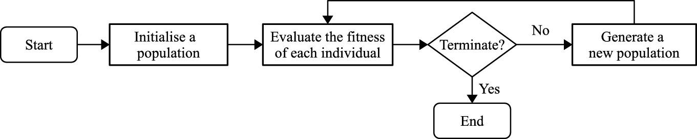
Outline of the main process of EC techniques
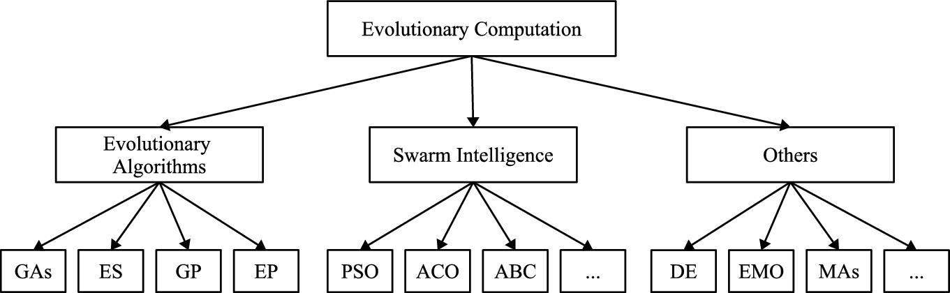
Categories of EC techniques
3.1.1 Evolutionary Algorithms (EAs)
EAs include GAs, GP, EP, and ESs, which are driven from the Darwinian principles. These four algorithms simulate the biological evolution process, where selection and genetic operators, i.e., reproduction, crossover and/or mutation, are used for generating new genetic materials/populations. The detailed introduction of GP is presented in Sect. 3.2. The other three algorithms are briefly described as follows.
3.1.1.1 Genetic Algorithms (GAs)
GA was the earliest EA proposed by Holland [33] in the 1960s and substantially extended by his students/colleagues and many important researchers [15, 48]. GA is the biggest branch of EAs with many well-known applications in optimisation problems, such as knapsack problems.

An example to show the representation of GA
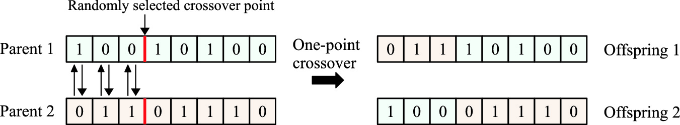
An example to show one-point crossover operation

An example to show mutation operation
3.1.1.2 Evolutionary Strategies (ESs)
In the 1960s, ES was proposed by Rechenberg [55]. Different from GAs, ESs consider both genotypic and phenotypic evolution, i.e., not only evolving genetic materials (building blocks) but also evolving a set of strategy parameters (or behaviour characteristics) [25]. Therefore, ESs have a different individual representation from GAs, which contains two parts, one part represents the genetic materials (building blocks) and the other part represents a set of strategy parameters, such as mutation step sizes [25]. The strategy parameters simulate the behaviour of the individual in its environment. The evolution of the genetic material is controlled by the strategy parameters. ESs use a similar evolutionary process as other EAs to search for the best solution based on selection and genetic operators. Different from GAs, ESs select individuals with better fitness to form the population in the next generation. In addition, ESs typically use self-adaptive mutation rates.
3.1.1.3 Evolutionary Programming (EP)
EP was introduced by Fogel [29] to evolve finite-state machines (FSM). Specifically, EP was employed to evolve programs to predict the next output symbol based on a set of previous symbols using a bit-based representation [29]. As an EA, EP is substantially different from GA, GP and ES. The main difference is that EP only uses the selection and mutation operators to generate a new population during the evolutionary process. The mutation operator in EP is often problem-specific in order to improve the fitness of the population. For example, a mutation operator with a self-adaptive step size may be employed in EP. Except for evolving FSM, EP can also be employed for function optimisation or other tasks.
3.1.2 Swarm Intelligence (SI)
SI indicates the collective behaviour of decentralized and self-organised swarms [38]. SI includes a group of EC algorithms driven from the social behaviours of animals, such as birds, ants, and bees. A swarm represents a collection of interactive individuals (organisms). SI algorithms simulate the collective behaviours of the individuals in the swarm to search for optimal solutions to problems. Representative SI algorithms include Particle Swarm Optimisation (PSO), Ant Colony Optimisation (ACO), and Artificial Bee Colony (ABC).
3.1.2.1 Particle Swarm Optimisation (PSO)


 and
and  represents the position and velocity of the ith individual in the dth dimension at the tth time (iteration/generation), respectively.
  and
and  indicates the ith particle’s pbest and gbest in dimension d at time t, respectively.
  and
and  are acceleration constants, which are important parameters in PSO.
  and
and  are randomly generated constants from an uniform distribution in dimension d at time t. The initial weight w indicates the impact of the last velocity on the current velocity, which is often a constant in a predefined range.
PSO was originally proposed for continuous variable optimisation, which is different from GAs for discrete variable optimisation. PSO has been successfully applied to many tasks, including function optimisation, parameter optimisation, scheduling, and feature selection [13, 51, 70, 71].
3.1.2.2 Ant Colony Optimisation (ACO)
ACO was proposed by Dorigo in 1992 [22]. Inspired by the foraging behaviours of the ant colony, the aim of ACO is to find the shortest path in a graph towards the food source. ACO uses a colony of artificial ants to search for the optimal path. Each ant represents a candidate path to a problem. At the initialisation step, each ant randomly constructs a solution (chooses a path) such as a collection of ordered edges in the graph. During the search process, each ant in the colony can drop a pheromone deposit on the path. The shorter path has stronger pheromone deposits, which could attract more ants to select this path. The pheromone deposits of all the edges are updated (increased or decreased) based on the time and the amount of pheromone deposited by each ant. A pheromone evaporation coefficient is employed to control the deceasing degree of pheromone deposit over time. After the search process, the shortest path found by the ant colony is returned.
ACO has been widely used to find optimal solutions for combinatorial optimisation problems, such as travelling salesman problem, routing, job scheduling, and graph colouring problems [23, 25].
3.1.2.3 Artificial Bee Colony (ABC)
ABC was proposed by Karaboa [35, 36] in 2005. ABC simulates the foraging behaviours of a bee swarm. In ABC, a swarm, containing a set of artificial bees, to search for the optimal solution (the best food source) through a number of iterations. In an ABC swarm, there are three types of artificial bees, i.e., employed bees, onlooker bees and scout bees. The employed bees search for food sources in the search space and share the food information with the onlooker bees. The onlooker bees receive the food information of all the employed bees and select one good food source. The scout bees are a small proportion of the employed bees that abandon their food sources and search for new food sources. In the search process, better food sources indicate that the solutions have better fitness.
ABC has been applied to various problems, such as engineering problems, feature selection, image preprocessing, and data mining [37].
3.1.3 Other Techniques
This group includes many well-known and important EC algorithms that do not belong to the previous groups, such as DE and EMO. This section briefly discusses these two algorithms.
3.1.3.1 Differential Evolution (DE)
 , with a dimension of n, an offspring
  is generated by randomly selecting three different individuals, i.e.,
  ,
,  and
and  , from the population. For the dth dimension of the individual
  , it is updated according to the followings.
![$$\begin{aligned} x^{t+1}_{i,d} ={\left\{ \begin{array}{ll} p^t_{i_3,d}+\gamma (p^t_{i_1,d}-p^t_{i_2,d}),&{}\text {if}~random[0, 1]<p_r \ or \ d=j,\\ x^{t+1}_{i,d},&{} Otherwise. \\ \end{array}\right. } \end{aligned}$$](../images/502867_1_En_3_Chapter/502867_1_En_3_Chapter_TeX_Equ3.png)
 .
. ![$$p_r \in [0, 1]$$](../images/502867_1_En_3_Chapter/502867_1_En_3_Chapter_TeX_IEq16.png) indicates the reproduction probability.
indicates the reproduction probability. ![$$\gamma \in [0, \infty ]$$](../images/502867_1_En_3_Chapter/502867_1_En_3_Chapter_TeX_IEq17.png) indicates a scaling factor.
indicates a scaling factor.With the above equation, each offspring is a linear combination of the three randomly selected individuals or inherits directly for its parents. This is similar to the crossover and mutation operations in EAs. In DE, if the offspring achieves better fitness than the parent, it will be selected for the next iteration. Otherwise, the parent will be selected for the next iteration.
DE has been applied to many optimisation problems in many fields, such as electrical power systems, electromagnetism, propagation, microwave engineering, control systems, and robotics [18].
3.1.3.2 Evolutionary Multi-Objective (EMO)


 indicates the ith objective function to be minimised (without loss of generality, a minimisation problem is considered here) and
  indicates the number of objective functions. x indicates a vector of decision variables. The constraint functions are
  and
and  , and the numbers of constraints are m and n, respectively.
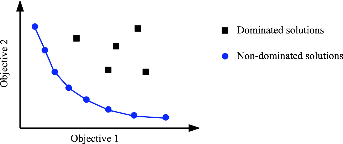
Pareto front (blue line) for a bi-objective minimisation problem
Many well-known EMO algorithms have been developed for multi-objective optimisation problems. These algorithms can be broadly classified into different groups [67], such as the methods using (relaxed) Pareto dominance relations, decomposition-based methods, reference set-based methods, and indicator-based methods. Representative EMO algorithms include Non-dominated Sorting Genetic Algorithm II (NSGA II) [20], Strength Pareto Evolutionary Algorithm 2 (SPEA2) [74], and MOEA based on Decomposition (MOEA/D) [72].
3.2 Genetic Programming
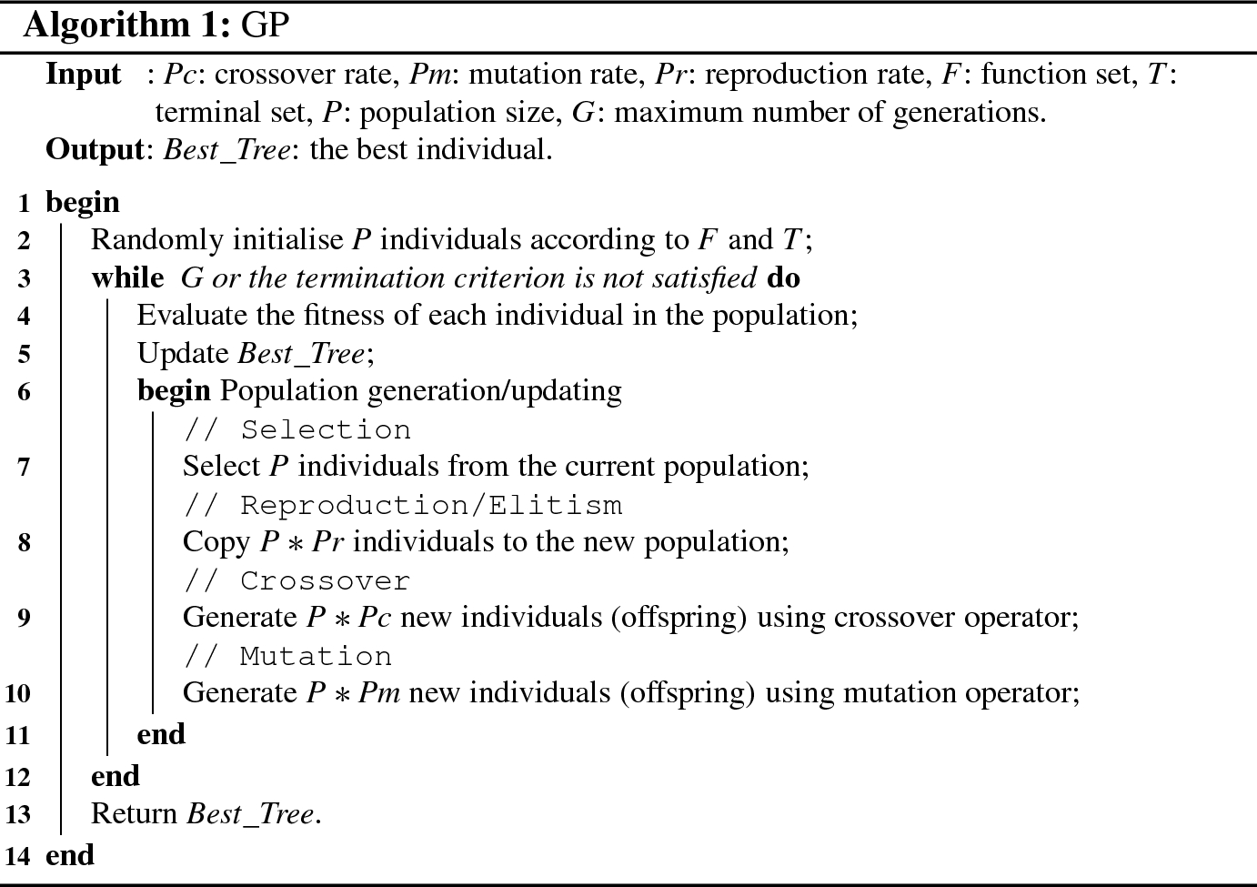
The flowchart of GP
3.2.1 Representation
There are several well-known GP variants with typically different representations, including Tree-based GP [40], Linear GP (LGP) [16, 17], Grammatically-based GP (or Grammar Guided-GP, GGGP) [68], and Cartesian GP (CGP) [47]. Among these versions, the most commonly used one is the tree-based GP [52]. This book employs tree-based GP to deal with image classification. For simplification, we use GP to indicate the tree-based GP.
 ,
,  ,
,  and
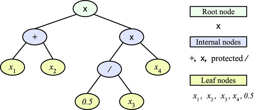
and  , and an Ephemeral Random Constant (ERC), i.e., 0.5. These variables/features and ERCs are called terminals of GP. The root node of this example tree is
  and the internal nodes are
  ,
,  , and protected /, which are called functions/operators of GP. A GP tree is often expressed in a prefix notation similar to the Lisp S-expression in the programming. For example, the example tree in Fig. 3.8 is expressed as
  , which can also be formulated as
  .
.
An example GP tree
The variable-length tree-based representation of GP is highly flexible and its structure can be easily adjusted according to the problems in hand. A good representation is expected to sufficiently represent the potential solutions of the problem and allows GP to effectively search for the optimal solutions. Thanks to its high flexibility, several variants of tree-based GP can be found from the literature, such as multi-tree GP and Strongly Typed GP (STGP). The details of STGP will be described in Sect. 3.3.
3.2.2 Terminals and Functions
To represent a GP tree, a function set
and a terminal set must be defined. A terminal set typically consists of variables/features/attributes and ERCs. The variables/features/attributes are related to the problem/task. For example, for a classification task, the terminal set may include the features of the dataset. The terminals represent the inputs of a GP system. Given an instance with a number of features, a GP tree can be executed by feeding the features of the instance in and return the output. Taking the GP tree in Fig. 3.8 as an example, if the values of  ,
,  ,
,  and
and  are given, the output of a GP tree can be calculated according to the corresponding expression.
A function set has functions used for building the internal and root nodes of GP trees. The functions are also related to the problem domain. In general, two types of functions can be used: general functions and domain-specific functions. General functions include arithmetic functions, i.e.,  , −,
, −,  , and protected division /, logical functions, such as if and or, and other functions, such as cos, sin, log, and exp. These functions take one, two or multiple arguments as inputs and perform corresponding operations on the inputs. These functions are commonly used to solve relatively simple problems, including feature selection, feature construction, classification, and symbolic regression. Domain-specific functions are the functions highly related to a specific domain, such as image domain. Domain-specific functions can be used to facilitate the solution representation in GP in order to find better solutions than using general functions.
The sufficiency and closure are two main criteria to construct/choose the function set and the terminal set for GP to solve a problem [40, 52]. Sufficiency indicates that the defined functions and terminals are sufficient to express a solution to the problem at hand. Closure includes type consistency and evaluation safety [52]. Type consistency means that the input and output types of functions are consistent. Evaluation safety avoids failures or errors generated by functions at run time. For example, the division is protected by returning zero or one if the divisor (the second argument) is zero in GP.
3.2.3 Population Initialisation
Similar to other EC techniques, the initial population of GP is typically randomly generated. Before population initialisation, the maximum tree depth is typically defined. The tree depth indicates the depth from the root node (starts from 0) to the deepest leaf node in the GP tree. There are three main methods to initialise a GP population, i.e., full, grow and ramped half-and-half [52].
The full method generates a population of trees where all the leaf nodes in the trees are at the maximum tree depth. In the full method, a tree is generated by randomly selecting functions from the function set as internal or root nodes. When reaching the maximum tree depth, the terminals selected from the terminal set are employed to form the leaf nodes. Figure 3.9 shows an example tree generated by the full method that all the leaf nodes are at the same depth of two.
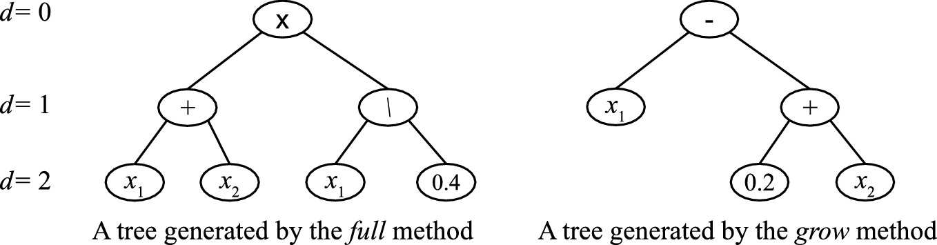
Examples to show the full and grow method. The maximum tree depth (d) is 2
The ramped half-and-half method is a combination of the full and grow methods to generate a population of trees. In the ramped half-and-half method, half of the population is generated by the full method and the remaining half of the population is generated by the grow method. This method ensures a wider range of sizes and shapes of the generated trees. The ramped half-and-half method is the most commonly used method for population initialisation in GP.
3.2.4 Fitness Evaluation
Fitness evaluation is an important component of the evolutionary process as it guides the search of GP to find better individuals. A fitness function is used to evaluate the fitness of each individual in the population. However, in many cases, choosing a good fitness function is not an easy task. A good fitness function will lead the search smoothly towards the best solution, while a bad fitness function would mislead the search. Typically, the fitness function is related to the problem being tackled. For example, for a classification problem, the commonly used fitness function is the classification accuracy [26].
3.2.5 Selection
In the evolutionary process, a selection method is employed to select individuals from the current population for genetic operators. Typically, an individual with better fitness has a larger chance to be selected. There are a variety of selection methods proposed and used, such as rank selection, fitness-proportionate selection and tournament selection [31, 32, 40].
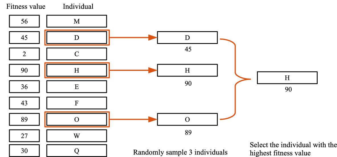
An example to illustrate tournament selection (size  3). A higher fitness value indicates an individual is better
3.2.6 Genetic Operators
An example to show the subtree crossover operation
An example to show the subtree mutation operation
- 1.
Reproduction: The reproduction operation is based on the trees selected by the selection method. It copies the selected trees (individuals) to the new generation. Since the majority of the selection methods are related to fitness, the reproduction operation allows the population to keep good trees in the new generation. Elitism is another strategy commonly used in GP for copying individuals to the new generation. In elitism, a small proportion of the best trees in the population are directly copied to the new generation.
- 2.
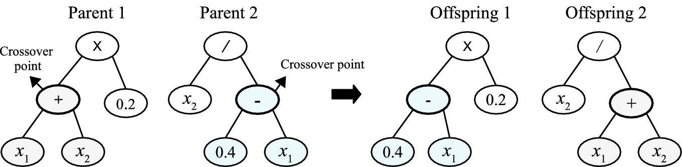
Crossover: The crossover operation is based on two selected trees (parents) to generate two new trees (offspring). In GP, the most commonly used form of crossover is subtree crossover [52]. Figure 3.11 shows an example of the subtree crossover operation, where two trees on the left are parents and two trees on the right are offspring. The crossover operation starts by randomly selecting two points in the parent trees and then swapping the subtrees according to the selected points to generate two new trees. The crossover operation attempts to generate good trees by recombination of the current genetic materials.
- 3.
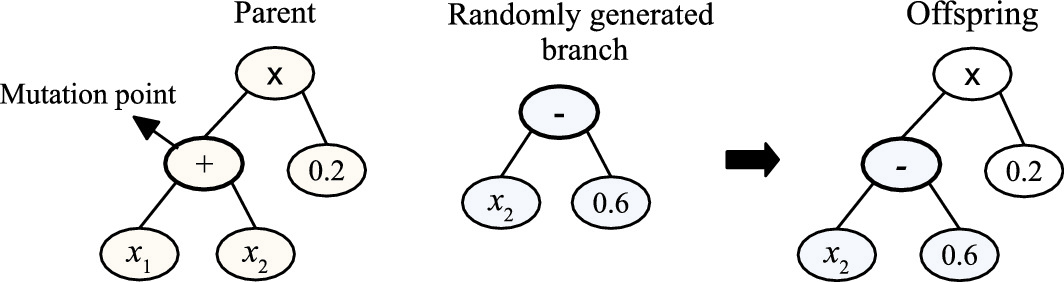
Mutation: The mutation operation generates a new tree based on one selected tree. In GP, the subtree mutation method is commonly used. The subtree mutation operation randomly selects a point of a tree and then replaces the branch rooted at this point with a randomly generated subtree to generate a new tree. Figure 3.12 shows an example of the subtree mutation operation, where tree on the right is the newly generated tree by mutation. In GP, the mutation operation is very important to maintain the diversity of the population because it introduces new genetic materials in the population.
3.3 Strongly Typed Genetic Programming
According to the closure criteria of functions, the traditional tree-based GP method only deals with one type of data, which limits the applicability of GP on complex problems that require multiple data types. To address this issue, a Strongly Typed GP (STGP) was proposed as an enhanced version of GP by Montana in 1995 [49] to handle data type constraints. In STGP, each terminal, e.g., features/variables or constant parameters, has an output type. Each non-terminal (function) has input types and an output type. The input type indicates the type of the argument of a function. The output type indicates the type of the value returned by a function/terminal. The input and output types limits a GP tree construction. For example, a function can only accept children nodes whose output types are the same as this function’s input types.
 ,
,  and
and  , and the terminals are
  ,
,  and
and  . These functions and terminals have types of Array1, Array2, Array3, Integer, Double1, and Double2. In the left branch of this example tree, the terminal
  has an output type of Double1. The function
  has an input type of Double1. Based on the type constrain, the
  terminal is used as the child node of
  . It is also noticeable that the
  function can only use the terminal
  as its child node from the current terminal and function sets. From this example tree, the constraints on the connections of different functions and terminals with different types can be easily found.
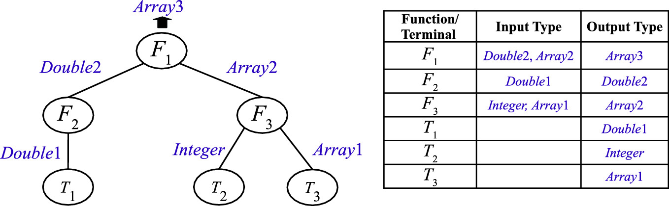
An example to illustrate the representation of STGP
In STGP, type constraints need to be satisfied in the initialisation step, the crossover and mutation operations. The three tree generation methods (full, grow and ramped half-and-half) can be used to build a population of GP. The tree generation starts from randomly selecting a function whose output type is the same as the output type of the GP tree to be the root node. Then based on the input types of the root node, the functions with the same types are selected to be the child/internal nodes. In the tree generation process, the type constraints have higher priority than the tree depth constraint. Therefore, a tree is built to meet the type constraints first and then the tree depth constraint. In the subtree crossover and mutation operations, the type constraint should also be satisfied. The subtree crossover operation performs on two subtrees of two parents with the same output types. The subtree mutation operation randomly generates a new branch with the same output type as that of the selected branch and replaces the selected branch.
In STGP, it is possible to employ different functions for special purposes according to the problem. In general, specific program structures are developed to integrate functions or terminals with different types into a single GP tree. The functions can be different types of domain-specific functions, such as image filtering functions and arithmetic functions. Compared with standard GP, STGP provides more possible ways to use different functions. STGP has been successfully applied to many tasks, including feature extraction [9], edge detection [30], and image classification [8, 14, 44]. The algorithms presented in this book are based on STGP. This book will provide more insights into how STGP with different representations are designed and implemented for dealing with image classification tasks.
3.4 Genetic Programming for Image Classification
This section reviews the closely related work on GP for image classification and the GP-based feature learning algorithms for other tasks.
Existing GP algorithms for image classification are broadly classified into three groups: (1) learning from pre-extracted image features, (2) learning from raw pixels/images, (3) evolving neural networks for image classification. Figure 3.14 shows the taxonomy of the related work. The embedded GP approach not only learns features but also constructs classifiers for classification. The wrapper GP approach is only used for feature learning and external classification algorithms are used for classification. Note that there are no existing works on the filter GP approach for feature learning because the aim of feature learning is to find better data representation to improve the classification performance and the filter GP approach does not necessarily improve the classification performance.
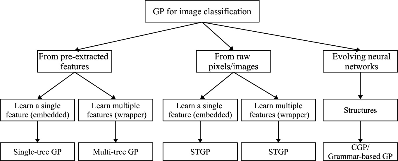
Taxonomy of existing GP algorithms for image classification
3.4.1 Learning from Pre-extracted Image Features
Nandi et al. [50] introduced a GP method for classifying breast mass into the benign and malignant classes based on the selected features. In the classification system, a number of Regions Of Interest (ROIs) were manually identified. Then 22 features, including four edge-sharpness measures, four shape factors and fourteen Grey-Level Co-occurrence Matrix (GLCM) features, were extracted from each ROI. Traditional feature selection methods, including sequential forward selection, sequential backward selection and student’s t test, were used to select a subset of features from the 22 features as inputs of GP, which was able to construct high-level features for classification. This method has achieved promising results in classification. However, this approach required domain experts to perform ROIs identification and estimate shape factors, which were not easy.
Ryan et al. [59] developed a system to detect the first stage of cancer where a GP method was used for mammographic image classification. A set of preprocessing operations, including background suppression, image segmentation, feature detection, and feature selection, were conducted for image classification. Two GLCM features, i.e., contrast and difference entropy of each segment, were manually selected as inputs of the GP system. This system has gained 100% accuracy on one dataset. However, this method requires domain knowledge to extract or select effective features.
Ain et al. [4] proposed a GP method for feature selection on skin cancer image classification. This method evolved classifiers based on 71 features, consisting of 12 domain-specific image features and 59 uniform Local Binary Pattern (LBP) histogram features. This method has also been analysed as a feature selection method. This method achieved significant or comparable performance on skin cancer detection than the other classification methods. However, this method needs domain knowledge to extract effective features from images for performing the task.
Ain et al. [6] developed a multi-tree GP method for skin cancer image classification. First, four different sets of features were extracted from the skin cancer images, including LBP features from the grey channel, LBP features from three colour channels, colour variation features of the lesion regions, and shape features of the lesion regions. Each individual of the multi-tree GP method had four trees and each tree constructed one high-level feature from a different set of features. In other words, each individual can produce four features, which were fed into different classification algorithms, including KNN, DT, MLP, RF, NB, and SVM, to perform classification, respectively. The results showed that the wrapper GP methods achieved better classification performance than single-tree GP wrapper and embedded methods, multi-tree GP embedded method, and classical classification algorithms on binary classification datasets. The effectiveness of these wrapper GP methods has also been verified on two multi-class skin cancer image classification datasets.
Ain et al. [5] further extended multi-tree GP to construct multiple features for skin cancer image classification. This method used five GP trees in an individual to independently construct features from five different types of pre-extracted features and used a classification algorithm for classification. This method has achieved better performance than the GP methods that construct one high-level feature and the other classification methods using different types of features on two skin cancer image datasets. Although these three methods in [4–6] have achieved promising results and showed relatively high interpretability, these methods have a limitation that requires domain knowledge and human intervention to extract effective features from images.
In summary, the aforementioned methods typically use a simple representation of GP but different features/inputs. These methods are easy to implement and often computationally efficient. However, the classification performance of these GP systems highly relies on the pre-extracted features. Generally, it is important to extract a number of task-specific features for improving the classification performance, such as the texture features for mammographic or dermoscopic images. Domain expertise is often needed for image preprocessing and feature extraction. In the next subsection, we will review typical work related to learning directly from image raw pixels for image classification using GP.
3.4.2 Learning from Raw Pixels/Images
3.4.2.1 Learning a Single Feature
Atkins et al. [14] developed a multi-tier GP method (simplified as 3TGP in [7]) to perform automatic feature extraction and image classification. Based on STGP, this method has three tiers, i.e., an image filtering tier, an aggregation tier and a classification tier, to process the input image, extract and construct high-level features for classification. Simultaneously, the evolved GP tree can be used as a classifier for binary classification by comparing the output value of GP with a predefined threshold. In the image filtering layer, several typical image filters, such as the mean filter, the max filter, and the min filter, were employed to process the input image. In the aggregation tier, small regions were detected and important pixel statistics of these regions were extracted. The extracted features were further constructed at the classification tier to be a high-level feature for classification. This method has achieved better classification performance than the other methods using manually extracted features on the face and pedestrian classification datasets.
Al-Sahaf et al. [7] proposed a two-tier GP (2TGP) method to image feature extraction and classification from raw images. Compared with 3TGP, the representation of 2TGP was simplified by only having the aggregation tier and the classification tier. Therefore, 2TGP could be faster than 3TGP. The results showed that 2TGP could achieve better or comparable results in several image classification datasets. Two variants of 2TGP were proposed in [8] to automatically detect more flexible shapes and sizes of regions, where features were extracted from. However, the performance of the 3TGP and 2TGP methods was only evaluated on binary image classification datasets.
A GP-HoG method was proposed by Lensen et al. [44] to employ the HOG descriptor as a function in 2TGP to achieve automatic region detection, feature construction, feature extraction, and image classification using raw images. From the automatically detected regions, this method extracted the specific histogram feature or distance features of HOG. The extracted features were further constructed for classification. The GP-HoG method demonstrated how the advanced HOG descriptor was integrated into GP to achieve high-level feature extraction and showed promising results in image classification. Compared with the 2TGP method in [7], the GP-HoG method has obtained better results on all the three datasets.
Evans et al. [27] proposed a GP method (ConvGP) with a convolution layer, an aggregation layer and a classification layer for image classification. The convolution layer has convolution and pooling operators. The parameters of the filters can be automatically selected by ConvGP. A single tree of ConvGP can simultaneously perform convolution, pooling, region detection, feature extraction, feature construction, and classification. The results showed that ConvGP achieved better classification performance than the other classification algorithms but worse classification performance than Convolutional Neural Networks (CNNs) with six layers on four binary image classification datasets.
Evans et al. [28] extended the ConvGP method by developing a memetic algorithm based on GP and gradient descent for image classification. This method had the same representation as ConvGP, but it used gradient descent to search for the best filters in the convolutional layer. With this local search operator, this method achieved better classification performance than ConvGP, but consumed much longer training time on four image classification datasets.
In summary, many GP methods have been developed to learn/construct one high-level feature for classification from raw images. These GP methods typically have a specific representation to perform multiple tasks using a single tree. The GP tree can also be employed as a classifier for binary image classification. These methods benefit from the flexible representation of GP and show a promise in image classification. A very good characteristic of these methods is that the evolved/learned programs/trees can be easily interpreted and many of the features constructed from the internal nodes are also understandable and can be re-used. However, these methods may not be effective for difficult image classification tasks by only learning one high-level feature. In addition, these methods have only been examined for binary image classification tasks. To deal with multi-class image classification tasks, many methods that can learn multiple high-level features have also been developed.
3.4.2.2 Learning Multiple Features
Shao et al. [60] proposed a multi-objective GP (MOGP) method to automatically learn multiple features from images for classification. MOGP has four layers, i.e., a data input layer, a filtering layer, a max-pooling layer, and a concatenate layer. Each layer employs a different type of functions for different purposes. MOGP simultaneously optimised two objectives, i.e., classification accuracy and tree size. In MOGP, a linear SVM was used to perform classification based on the learned features. The results showed that MOGP obtained better performance than several traditional feature extraction methods and a five-layer CNNs on four different image classification datasets. However, MOGP could produce a large number of features from an input image. Additionally, this method has a very complex feature learning process, which is computationally expensive.
Liu et al. [46] proposed a GP method to learn spatio-temporal motion features for action recognition. The idea behind this method was similar to that in [60], while this method used 3D sequence as inputs and employed a number of functions/operators for video processing in its filtering function set. In addition, this method only employed the max pooling function in the pooling layer. The results showed that this method obtained better performance than CNNs and Deep Belief Networks (DBNs) on several well-known datasets. This method also showed good interpretability and understandability.
Agapitos et al. [1] developed a layer-wise GP method for handwritten digits recognition. This method has a filter bank layer, a transformation layer, an average pooling layer, and a classification layer. Specifically, the filter bank layer has a collection of filters to convolve the input image. Similarly, Suganuma et al. [64] developed a GP method by using more layers with filters for feature learning. This method has two stages of feature learning, where the first stage uses a combination of image processing filters and the second stage uses a combination of evolved filters. These two methods have similar solution structures to that of CNNs, but they have not been compared with CNNs.
Al-Sahaf et al. [9] proposed a GP method to automatically evolve rotation-invariant texture descriptors for texture classification with a small number of training instances. This method used a procedure similar to LBP to generate a feature vector from an image using a sliding window. The evolved GP descriptor is a classical GP tree, consisting of the arithmetic functions as internal/root nodes and the pixel statistics of the sliding window as leaf nodes. The employed pixel statistics are the mean, max, standard deviation, and min values of a sliding window, which allows the learned features to be rotation-invariant. With a distance-based fitness function, this method could learn effective features from a small number of training instances. The results showed that this method achieved better performance than using existing texture descriptors (e.g., LBP, GLCM and other LBP variants) for texture image classification.
Al-Sahaf et al. [10] developed a dynamic GP method to generate a flexible number of texture features for classification, which addressed the limitation of the method in [9]. Several root nodes with a flexible number of children nodes were developed in this approach to allow it to produce variable lengths of features. The results showed that this method achieved better performance than the method in [9] by learning a flexible length of features. However, these two GP descriptors inspired by the LBP descriptor were originally proposed for describing texture features, which might not be effective for other types of image classification tasks.
Price and Anderson [53] designed a GP method for image feature descriptor learning and applied multiple kernel-learning SVM for classification. This method employed a set of image operators, such as Canny, Hough Circle and Harris Corner Detector, as functions to learn image descriptors. The results demonstrated that this method achieved promising classification performance on one dataset. However, this method should be examined on more image classification datasets to show its effectiveness. In addition, many other image-related operators can be employed in GP to learn effective features, which has not been comprehensively investigated.
Price et al. [54] further improved the method in [53] by developing a new GP method to improve the search ability to learn effective features for image classification. This method had a set of image operators as functions and grey, red, blue, and green images as terminals. New crossover and mutation operators were introduced in this method to control the bloat of GP and improve the diversity of the population. The results showed that this method achieved better classification performance on a difficult scene classification dataset than a CNN-based method.
Iqbal et al. [34] developed a GP method with transfer learning for complex image classification tasks. The building blocks of GP trees evolved from a source task were extracted and reused in GP to deal with another similar or different task. This method investigated the use of the extracted knowledge in the process of individual initialisation and mutation operation. The extensive results showed that transfer learning can be employed to improve the performance of GP crossing different image classification tasks, including texture classification and object classification.
Almeida and Torres [12] proposed a GP method to evolve effective similarity functions from a set of existing functions in remote sensing image classification. The evolved GP tree transformed time series raw pixels into a set of features to form the dissimilarity matrix, which were fed into KNN for classification. Compared with the commonly used methods that used existing similarity functions, the GP method achieved better performance in remote sensing image classification.
To summarise, many GP methods have been proposed to automatically learn multiple features for image classification from raw images. These methods have specific GP representations (program structures, function sets and terminal sets) that define how features are learned from the images. These methods could automatically extract informative features from the task being tackled and achieve promising performance in image classification. The solutions evolved by these GP methods also provide potential interpretability in what and how the features are extracted or learned from the images, and why they are effective for classification. GP has a flexible representation, indicating that there are many possible ways to learn effective features. However, this has not been comprehensively investigated. In addition, most of these methods have only been applied to limited types of image classification tasks. The potential of GP in feature learning for different image classification tasks has not been comprehensively investigated.
3.4.3 Evolving Neural Networks for Image Classification
Suganuma et al. [65] proposed a GP method to automatically evolve architecture of CNNs (CGP-CNNs) for image classification. This method was based on Cartesian GP (CGP). A set of commonly used functional models of CNNs, including convblock, resblock, max pooling, average pooling, summation, and concatenation, were designed as GP functions. In CGP-CNNs, each GP individual represents a CNN with a specific architecture, which is trained via backpropagation using gradient descent for image classification. The results showed that CGP-CNNs achieved similar or competitive performance but found models with slightly less parameters compared with the state-of-the-art CNNs. However, this method is computationally expensive.
Zhu et al. [73] proposed a tree-based GP method for evolving architectures of CNNs for image classification. The leaf nodes of a GP tree were the resblock and the internal or root nodes were normal functions for block assembling. This approach benefits from the flexible representation of GP to evolve solutions with a variable length/depth. A dynamic crossover operator was developed in this method. The results showed that this method achieved results competitive with the state-of-the-art automatic or semi-automatic neural architecture search algorithms on the well-known CIFAR10 dataset. Compared with CGP-CNNs, this method has achieved better classification but found models with more parameters.
Diniz et al. [21] designed grammar-based GP to find the architectures of CNNs for image classification. This method used simple grammar to encode an architecture of CNN that consists of convolutional layers, pooling layers and fully connected layers. This method has been examined on the CIFAR10 dataset and compared with another automatic neural architecture search method. However, this method only searched simple connections of the different layers and cannot search for optimal values for the parameters in the layers, including the number of filters and the kernel sizes.
To sum up, these existing works showed the promise of using GP to evolve CNNs for image classification. However, there are very few works in this field, which due mainly to the high computational cost. In addition, the CNNs methods mainly focus on large-scale object classification benchmark datasets, i.e., CIFAR10 and CIFAR100, with a huge number of instances [41]. However, there are many other image classification tasks in the real world. It is necessary to develop new GP-based approaches for different types of image classification tasks.
3.4.4 GP for Feature Learning in Other Tasks
Rodriguez-Coayahuitl et al. [56] developed a GP method to learn effective and deep representations of data in a way that is similar to neural networks. This method employed GP forests of standard trees to learn a set of features from raw images. This method has multiple structured layers to learn deep representation. Specifically, an encoder forest and a decoder forest was employed to learn a representation in a way that is similar to auto-encoder. The GP auto-encoder was further investigated in [58], where GP auto-encoder with an online learning method using different population dynamics and genetic operators was proposed. The reconstruction performance of this method has been extensively investigated on image datasets. However, these methods could be employed to deal with many other tasks, such as image classification and object detection, to further demonstrate its effectiveness on representation learning.
Rodriguez-Coayahuitl et al. [57] proposed a convolutional GP method to automatically evolve filters for image denoising, where each GP tree can be employed as a filter to convolve the image. This method can have one layer to construct one filter or have multiple layers to generate multiple filters to convolve the image sequentially. The idea of this method is similar to CNNs, but the filters generated by this method are different from those in CNNs. However, the performance of this method has only been examined on image denoising, although this method achieved better performance than a denoising CNN method.
Liang et al. [45] applied GP to construct high-level features for figure-ground segmentation from seven different types of features, respectively. A GP tree could be used as a classifier to classify the pixel of an image into the object and non-object classes. The effectiveness of the GP methods with different terminal sets were investigated and compared. The results showed that the GP methods could achieve better results than four conventional segmentation techniques on different datasets.
Tran et al. [66] proposed GP methods to automatically construct multiple class-dependent and class-independent features from high-dimensional data for classification. The fitness functions were developed in GP to construct class-dependent and class independent features, respectively. Multi-tree GP was employed to construct multiple features for classification. The results showed the effectiveness of GP-based feature construction for high-dimensional classification. However, these methods only learned a fixed number of features, which may not be the optimal set of features for a classification task.
La Cava et al. [43] developed a multidimensional GP method with Lexicase selection and age-fitness Pareto survival to automatically learn multiple features using a stack-based representation. In the stack-based GP, each individual produced multiple features. Based on the learned features, the nearest centroid classifier was employed for classification. The results showed that this method achieved better performance than many classification algorithms. However, this method could learn a small number of features.
Wu et al. [69] applied GP to automatically evolve image descriptors that can extract features from various images for image registration. This GP method employed a set of simple arithmetic operators as functions and the statistics of the region as terminals to evolve descriptors, which can reduce noise interference of images. The results showed that this method achieved better performance than the other four descriptors and one GP method on five datasets.
La Cava and Moore [42] proposed a multi-objective multidimensional GP method to learn effective features for symbolic regression. In the multidimensional GP, each individual produced a set of features. Then the learned features were weighted to form a linear model for symbolic regression. In this method, new genetic operators were developed to improve the learning performance. The results showed the effectiveness of this method over the other baseline methods on a large number of regression problems.
Fu et al. [30] developed several GP methods to automatically extract edge features from the images. Based on raw pixels, GP was able to construct low-level, Gaussian-based and Bayesian-based edge detectors, respectively. The results showed the effectiveness and potential interpretability of the GP methods on edge detection.
Besides, GP has also been successfully applied to many other tasks. Recent reviews on related works can be found in [2, 3, 11]
3.5 Summary
This chapter reviewed the main concepts of evolutionary computation and genetic programming. This chapter also reviewed and discussed the related works of GP on feature learning for image classification and summarised the limitations of the existing works that form the motivations of this research. The following chapters (4–9) of this book will develop different GP algorithms to address these limitations.