7

Dance of the Digits

Dancing in all its forms cannot be excluded from the curriculum of all noble education: dancing with the feet, with ideas, with words, and, need I add that one must also be able to dance with the pen?

—Friedrich Nietzsche, German philosopher, poet, classical philologist1

If this book represents a journey passing through mountainous terrain, then this chapter represents one of the highest pinnacles that we shall attain. With many peaks, the toughest part of the climb is often the last part. In this vein, this chapter involves a bit more symbolic manipulation than some of the others—but it is still within your purview. I urge the less mathematically inclined of you to stay the course here. We have covered a lot of conceptual terrain to get to this point and now have placed within sight a much deeper understanding of how the modern methods of multiplication taught in the schools really work. Let us not now shirk from the symbols when we are so close. Hopefully you will find the scramble up this last segment of the trail illuminating (if needed, please visit www.howmathworks.com to see more examples).

The major focus of the previous chapter was to show that it is possible, in writing, to solve problems that require repeated addition by actually getting around doing all of those additions on paper. This allows us to significantly reduce the time it takes to find solutions in these situations—once more placing before us the universal idea of substituting one thing for another to gain decisive advantages. Due to its widespread occurrence, the name “multiplication” was given to this way of reckoning.

While much progress has been made in taming this operation (the Egyptian method of doubling, for instance), our times table methods in HA script are still not complete. Presently, we can only handle a restricted class of problems—namely, those involving an arbitrarily long number multiplied by a single digit. Computing such multiplications, in principle, has been completely solved and can usually be performed much faster, with times tables, than using the Egyptian technique. But there are many, many other multiplications where both numbers have two or more digits (the five original problems of the last chapter, for instance) and the time has come to learn how to deal with these.

Additionally, we still need to see if the entire process can be miniaturized further into a single diagram in a manner similar in spirit to the compact algorithms we have for addition and subtraction.

Our goals then are this: to develop a general recipe (in HA script) that works for the multiplication of any two whole numbers, not just the special cases of the previous chapter, and then to stylishly simplify it. We will accomplish both in this chapter, and in the demonstration will see the overwhelming power inherent in the symmetry of the HA notation. This symmetry will give us the ability to take the repeated addition of a number and radically transform it into something completely different, into something that in its most expressive form can be likened to a drill team of digits marching to well-scripted rules—a veritable dance of the digits, if you will. This transformation, this poetry of the diagrams, allows for the operation of multiplication, which is significantly harder than either addition or subtraction, to be wrestled out of the hands of the specialist and laid at the doorstep of elementary school-aged children.

Carving Up the Numerals

The plan of attack, when multiplying two numbers in HA script, is to “carve up” the multiplication or product in a way that allows us to unleash the times table on it. When the product is of the form “two or more digits × a single digit,” as in the last chapter, we break up the larger number to accomplish this (e.g., in 62 × 7 we split up the 62 [as 60 + 2] to get 60 × 7 + 2 × 7). However, if both numbers in the product contain two or more digits, we have some freedom in how we choose to decompose. For example, when computing the product 62 × 37, we can choose to carve up the 62 first or the 37 instead. To successfully handle these cases requires that we relocate the trailing zeros in the product.

If a numeral ends in one or more zeros, we will call these zeros “trailing zeros.” For example, 50 has one trailing zero and 500 has two trailing zeros. The numeral 100020 has four total zeros, but only the one at the end qualifies as a trailing zero. In HA script, trailing zeros are like free agents which can roam at will from the tail of one numeral in the product to the tail of the other. The following all show that while the total number of trailing zeros is conserved in the product (before completing the multiplication, that is), they can move freely between either numeral:

 

One Trailing Zero: 60 × 1 = 6 × 10 = 60

 

Two Total Trailing Zeros: 60 × 10 = 6 × 100 = 600 × 1 = 600

 

Four Total Trailing Zeros: 600 × 700 = 60 × 7000 = 6000 × 70 = 6 × 70000 = 420000

 

Five Total Trailing Zeros: 54000 × 7200 = 54 × 7200000 = 5400 × 72000 = 5400000 × 72 = 388800000

 

In terms of our viewpoint of multiplication as repeated addition, these seemingly innocuous shifts of zero are actually tremendous simplifications. They have far greater impact on reducing the number of additions required than even does simply reversing the order of the multiplication. For instance, 600 × 700 means to take six hundred 700s and add them together. But by shifting zeros, we can swiftly rewrite this as 6 × 70000 and find the answer by knowing only that 6 × 7 is 42 and then putting the four zeros after it to obtain 420000—meaning in this case, that the collective effect of hundreds of additions has been rerouted to a single calculation that can be completed in less than ten seconds! These shifts play out on abacus rods as shown:

 

 

600 × 7 0 0 = 6 × 7 0 0 0 0 = 4 2 0 0 0 0

 

Exploiting the free agent properties of trailing zeros will prove to be pivotal to all that follows in that we can reposition them to convert multiplications between any two numbers, into multiplications found in the multiplication table. We just have to learn how to incorporate all of the shifts in such a way that everything aligns correctly—historically, no small task. If there are still any lingering doubts on the significance of the number zero (and the symbol representing it) to how we perform arithmetic, please let them cease here.

Nontrailing zeros, on the other hand, are bound and cannot be moved around at will since doing so gives different answers. For example, the zeros in the product, 7202 × 6008, are nontrailing and cannot be shuffled around: 7202 × 6008 ≠ 7220 × 6800.

To get the ball rolling let’s look at how the multiplication of “two digits × two digits” plays out by walking through “62 × 37”:

 

Carving Up Sixty-Two First (60 + 2)

62 × 37	=	60 × 37	+	2 × 37
Add 62		Add 60		Add 2
37s		37s		37s
		B	+	A

 

• A = 2 × 37:

In this form we still can’t directly engage the multiplication table. We must also split up the 37 (as 30 + 7) which gives: 2 × 37 = 2 × 30 + 2 × 7.

Now we can directly engage the table.

The fundamental patterns from the times table are: 2 × 3 = 6; 2 × 7 = 14

Using these patterns gives: 2 × 30 + 2 × 7 = 60 + 14 = 74.

And we have 2 × 37 = 74.

• B = 60 × 37:

In the form 60 × 37, we can’t directly engage the multiplication table. We must first reposition the trailing zero:

 

60 × 37	=	6 × 370
		Moving the trailing zero to the right

 

Decomposing the 370 (300 + 70) allows us again to engage the multiplication table:

 

6 × 370 = 6 × 300 + 6 × 70 = 1800 + 420 = 2220

The fundamental patterns from the times table are: 6 × 3 = 18; 6 × 7 = 42.

Adding the result in A to the result in B vertically:

 

74

+ 2220

2294

 

This gives 62 × 37 = 2294.

 

Carving Up Thirty-Seven First (30 + 7)

Since the order in which we multiply doesn’t matter (i.e., 62 × 37 = 37 × 62) we can read 62 × 37 from right to left (as 37 times 62). This interprets as adding together thirty-seven 62s:

 

62 × 37	=	60 × 30	+	62 × 7
Add 37		Add 30		Add 7
62s		62s		62s
		B	+	A

 

• A = 62 × 7:

As before, we can’t directly engage the multiplication table using the form 62 × 7. We need to also decompose 62 (60 + 2) which gives:

 

62 × 7 = 60 × 7 + 2 × 7 = 420 + 14 = 434

 

Thus 62 × 7 = 434.

The fundamental patterns used from the times table are: 6 × 7 = 42; 2 × 7 = 14

• B = 62 × 30:

Similarly in the form 62 × 30, we can’t directly engage the table. We must first reposition the trailing zero:

 

62 × 30	=	620 × 3
		Moving the trailing zero to the left

 

Now we decompose the 620 (600 + 20) which gives:

 

620 × 3 = 600 × 3 + 20 × 3 = 1800 + 60 = 1860

 

Thus 62 × 30 = 1860.

The fundamental patterns used from the times table are: 6 × 3 = 18; 2 × 3 = 6.

Adding the results in A to the result in B vertically:

 

434

+ 1860

2294

 

This gives 62 × 37 = 2294.

 

We obtain the same value of 2294 whether we decompose the 62 first or the 37 first. Regardless of which number we choose to break apart first, we end up carving up the other one as well. Breaking up both numbers is necessary to fully engage the times table.

Trailing Zeros Go to Work

We are on the scent of something significant here. To get a better feel for exactly what that is let’s give ourselves a longer piece of rope to play with this time by looking at the multiplication of 745 × 289:

 

Decomposing the 289 first:

745 × 289	=	745 × 200	+	745 × 80	+	745 × 9
Add 289		Add 200		Add 80		Add 9
745s		745s		745s		745s

Decomposing the 745 first:

745 × 289	=	700 × 289	+	40 × 289	+	5 × 289
Add 745		Add 700		Add 40		Add 5
289s		289s		289s		289s

To engage the multiplication table requires that we eventually take apart both numbers, the 745 next in the first case (to 745 = 700 + 40 + 5) or the 289 next in the second case (to 289 = 200 + 80 + 9). Once we have done both decompositions it then becomes a game involving only trailing zeros as indicated here:

 

745 × 289	=	745 × 200	=	700 × 200	+	40 × 200	+	5 × 200	(1st row)
	+	745 × 80	=	700 × 80	+	40 × 80	+	5 × 80	(2nd row)
	+	745 × 9	=	700 × 9	+	40 × 9	+	5 × 9	(3rd row)

or,

745 × 289	=	700 × 289	=	700 × 200	+	700 × 80	+	700 × 9
	+	40 × 289	=	40 × 200	+	40 × 80	+	40 × 9
	+	5 × 289	=	5 × 200	+	5 × 80	+	5 × 9

 

Notice that each of the nine partial products in the first product (745 × 289) are present in the second product (745 × 289) as well. In fact, the rows in the first product become the columns in the second product (e.g., the three partial products in the first row of the first product, 700 × 200 + 40 × 200 + 5 × 200, become the first vertical column in the second product) and vice versa (this is the transpose again). As a result of this equivalence, we need only use one of the two diagrams as we continue (we choose the first one with the labeled rows).

Now that we have taken apart both numbers completely, it becomes possible to fully engage the multiplication table for every product by simply repositioning the trailing zeros:

 

745 × 289	=		(7 × 2) 0000	+	(4 × 2) 000	+	(5 × 2) 00	(1st row)
		+	(7 × 8) 000	+	(4 × 8) 00	+	(5 × 8) 0	(2nd row)
		+	(7 × 9) 00	+	(4 × 9) 0	+	(5 × 9)	(3rd row)

Sum of Fundamental Products for 745 × 289

 

The fundamental products from the multiplication table are now: {7 × 2, 4 × 2, 5 × 2, 7 × 8, 4 × 8, 5 × 8, 7 × 9, 4 × 9, 5 × 9}. Computing these gives:

 

745 × 289	=		140000	+	8000	+	1000
		+	56000	+	3200	+	400
		+	6300	+	360	+	45

 

Adding these all up gives 745 × 289 = 215,305.

The systematic idea then is this: to fully break apart both numbers in a product, no matter how many digits, until we get down to single digits followed by trailing zeros. It is always possible to drill down a product this way in HA script. Once accomplished, it then becomes possible to fully engage the multiplication table (by simply repositioning trailing zeros) to find all of the partial products and then we complete the additions for the final answer.

There are patterns galore here and nowhere is that better demonstrated than in the “Sum of fundamental products for 745 × 289” expression. The following table makes these patterns explicit by listing the number of trailing zeros in each partial product entry with its accompanying coin denomination:

 

Zero Counts for 745 × 289

 

 

 

The pattern is the same whether we read the table horizontally or vertically (i.e., turning the rows into columns or vice versa yields the same arrangement). Is it possible to capitalize on these patterns? Most definitely!

Our next task then is to engineer a way to take advantage of these symmetries and translate this entire way of multiplying into a simpler, more convenient form.

Multiplication on Diagrams

The breakdown of 745 × 289 (into nine partial products involving the multiplication of single digits and trailing zeros) is general and will work in principle for the multiplication of any two whole numbers. And though it represents another triumph over brute force repeated addition (i.e., we can find 745 × 289 this way by doing far fewer than 289 additions), the method is still bulkier than we’d like and nowhere near as simple as it can be. We have seen that a very compact algorithm is possible in addition (shown here), and it is natural to ask if such a thing is possible with this type of multiplication.

 

Expanded addition versus compact addition (742 + 659):

 

Expanded Addition:

 

	(700	+	40	+	2)
+	(600	+	50	+	9)
	1300	+	90	+	11	=	1401

 

Compact Addition:

 

11

742

+ 659

1401

 

To obtain a recipe which is similar in spirit to compact addition, we will work from the table listing the count of zeros (for 745 × 289). A major obstacle in trying to acquire conceptual leverage over HA procedures is that we use the same symbols repeatedly in different locations or place values. This makes it very easy to get confused and lose track of what is really going on (is that really a 4000 or should it be 400 and how does it align).

With HA numerals, the positions of digits within a given string of numerals are how we distinguish place values. Coin numerals, on the other hand, allow us to distinguish different locations or place values by using different denominations; meaning that the coins can act as tracking devices, if needed, and this can turn out to be conceptually very useful—especially for multiplication and division. Let’s now exploit this to the hilt.

To keep everything tidy for our present purposes, we will represent the coin numerals without circles (including only the content of their value). Which means that throughout the rest of the chapter, we will characterize the coin numerals, and , respectively, by the letters “T” and “H.” Looking at the “Zero Counts Table for 745 × 289” and retaining only the coin information we obtain:

 

Zero Counts for 745 × 289—Coins Only

 

 

 

Before analyzing this table further, it can be helpful to use this diagram as a road map of sorts for multiplication. A road map gives us a convenient and useful model of a three-dimensional landscape. Convenience comes from the fact that it is astronomically easier to lay a road map, say of the state of Texas, in our lap than it is to do so with the actual material state (all 268,000 square miles of it).

Utility comes from knowing that, even though a lot of information gets lost in representing such a landscape on small sheets of flat paper (i.e., we do not know what a region really looks like, smells like, or feels like by reading such a road map), key structural information, nonetheless, is still captured (items such as names and numbers of roads, which roads go through which towns, which roads connect to other roads, what are the main roads, and so on). In most cases, this information turns out to be precisely what drivers need to successfully navigate through a part of the country that they have never been in before. Exploiting road maps in this way is no trivial matter to any who have used them to travel.

Now in a similar fashion, these coin diagrams will provide useful insight into the world of multiplication—insights allowing us to “navigate” our way to powerful procedures for performing the operation.

Notice in the previous table that the denominations can be aligned if we look at them diagonally from right to left:

 

Demonination Alignment for Zero Counts—Coins Only (745 × 289)

 

 

 

This alignment is what we will build from to construct the first of the miniaturized methods allowing us to tame the multiplication of whole numbers. To make it work, requires we use the following table showing how the coin denominations (place values) multiply among themselves:

 

Multiplication Table for Coin Denomnation or Place-Values

 

 

aT × H = 10 × 100 = 1000 = TH

 

We will now demonstrate how all of the pieces fit together by looking at the multiplication of 745 × 289 on the following sequence of grids:

 

A: Blank Grid

 

 

 

B: Place Values Written as Products

 

 

 

C: Place Values Multiplied (i.e., H × T = TH, etc.)

 

 

 

The sequence of steps A, B, C have gotten us back to the “Zero counts table for 745 × 289 – coins only” but this time in three steps, as opposed to the slower method in the previous section involving the repositioning of trailing zeros. Now we can multiply each of the individual digits directly on the table as follows:

 

D: Digits with Place Values Multiplied

 

 

a 4 T × 2 H = (4 × 2) (T × H) = 8 TH

 

E: Simplified Multiplications

 

 

 

The fundamental products used to multiply 745 × 289 on the diagram here, {7 × 2, 4 × 2, 5 × 2, 7 × 8, 4 × 8, 5 × 8, 7 × 9, 4 × 9, 5 × 9}, match those used in the previous section. Note that the same denominations occur on the diagonals (reading from right to left). Adding like denominations or place values gives:

 

						14 TTH	140000
		8 TH	+	56 TH	=	64 TH	64000
10 H	+	32 H	+	63 H	=	105 H	10500
		40 T	+	36 T	=	76 T	760
						45 1	45
							215,305

 

And the answer we obtain matches our result in the previous section for 745 × 289.

The “Sum of fundamental products for 745 × 289” diagram, which involved nine partial sums has now been road-mapped to nine entries in a table. The only difference between the two is appearance and how we get to them. The essential information is all the same with the same fundamental products from the times table being used in both cases. There is nothing that prevents all of the steps in the diagrams A–D from being compressed into the last diagram shown in E.

We demonstrate this by multiplying 452 × 78 on a single table (remembering to multiply both the digits as well as the place values):

 

 

 

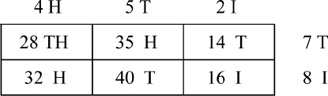
The fundamental products used from the multiplication table are: 4 × 7 = 28, 5 × 7 = 35, 2 × 7 = 14, 4 × 8 = 32, 5 × 8 = 40, 2 × 8 = 16.

Adding like place values along the diagonals gives:

 

				28 TH	28000
35 H	+	32 H	=	67 H	6700
14 T	+	40 T	=	54 T	540
				16 1	16
					35256

 

Thus 452 × 78 = 35256.

 

Now we have the makings of a time and space saving procedure. We start it off by performing fundamental multiplications on a diagram. The entries in the diagram naturally separate the partial products by place values. After this, we simply pluck the entries off the table like fruit, adding them together, and we are done.

In spite of this simplification, the procedure is still not as elegant as it can be. Right now we have a hybrid method using both HA numerals and coin numerals. The coins have been used much like conceptual boosters to add insight. Are we now stuck with them or can we jettison them, à la NASA, and develop an algorithm that only uses HA script?

The Lattice Method

The time has come to let the numerals dance. It turns out that HA numerals can dance in many ways. The remainder of the chapter is devoted to the discussion of two such routines.

Let’s begin by looking at the diagram corresponding to multiplying 23 × 56:

 

 

 

Plucking the entries from each of the blocks and adding yields:

 

				10 H	1000
15 T	+	12 T	=	27 T	270
				18 I	18
					1288

 

Rather than adding the same place values to each other first, we can instead keep each entry from the table separate and add them vertically:

 

10 H	=	1000
15 T	=	150
12 T	=	120
18 I	=	18
		1288

 

Now notice that each of the hybrid entries on the left can be simplified first by carrying; that is, 10 “H” (ten hundreds) can be simplified to 1 “TH” (one thousand) and 12 “T” (twelve tens) can be simplified to 1 “H” and 2 “T” (one hundred, two tens). Let’s see what happens if we put these changes in first before adding:

 

10 H	=	1 TH	0 H
15 T	=		1 H	5 T
12 T	=		1 H	2 T
18 T	=			1 T	8 I
		1 TH	2 H	8 T	8 I

 

The answer matches what we had previously, as it should, since we are only reorganizing the sums and not changing the values. Now observe what happens on the diagram for 23 × 56 if we do these simplifications first:

 

 

 

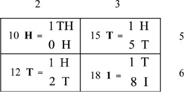
Judiciously reorganizing in each cell gives:

 

 

 

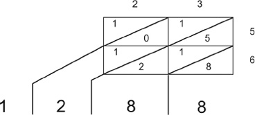
Things are aligned quite nicely now. If we draw a diagonal in each rectangle, we can see just how aligned the coin values have become.

 

 

 

The same denominations lie in the same lanes. In this format, we will be able to simply add the numbers in each lane to obtain the total amount we have for each place-value denomination. Extending the lanes and adding yields:

 

 

 

If we read the grid from right to left, we observe that:

 

The ones denomination is in the first lane.

The tens denomination is in the second lane.

The hundreds denomination is in the third lane.

The thousands denomination is in the fourth lane.

 

Given that the lanes become place values when extended, the above translates to:

 

The ones sum is in the first location or the ones place.

The tens sum is in the second location or the tens place.

The hundreds sum is in the third location or the hundreds place.

The thousands sum is in the fourth location or the thousands place.

 

This perfect alignment let’s us completely drop the coin tags and simply work with the numerals themselves:

 

23 × 56 (No Coin Tags)

 

 

 

The advantage of this last procedure is that it uses HA symbols alone—the conceptual coin tags have been jettisoned! Our goal of obtaining a miniaturized and efficient algorithm using purely HA script has been achieved.

Let’s demonstrate this procedure by multiplying 852 × 74:

 

852 × 74 (Blank Lattice)

 

 

 

Placing the diagonal lines in for each cell gives:

 

852 × 74 (Blank Lattice & Diagonals)

 

 

 

The products we have to consider from the times table of chapter 6 are:

 

Top row: 8 × 7 = 56, 5 × 7 = 35, 2 × 7 = 14

Bottom row: 8 × 4 = 32, 5 × 4 = 20, 2 × 4 = 8

 

Placing these products into their proper positions in the lattice yields:

 

 

 

Extending the lanes, adding (from right to left), and carrying (indicated by the 1s outside the squares) in formation gives:

 

 

 

Thus 852 × 74 = 63048.

This can all be done on a single diagram. Doing so for our signature multiplication of the chapter (745 × 289) gives:

 

 

 

And we have 745 × 289 = 215305. Compare this to all of our earlier methods of calculating this product.

This then is the lattice method of multiplication. It allows for the complete transformation of the problems of repeated addition into a procedure in writing that involves placing numbers into formation, via a multiplication table, and simply adding them along the lanes. It is as if the numbers have become part of a dance troupe routine, a routine in which we are able to accomplish the net effect of hundreds upon hundreds of additions in the span of less than a minute. Let’s now go back to the problem of finding the combined income of a country of 26,784,000 residents where each earns $17,200:

We must calculate 26,784,000 × 17,200.

Repositioning trailing zeros yields: 26,784 × 17,200,000 = (26,784 × 172) 00000.

We now use the lattice to calculate 26,784 × 172:

 

 

 

Thus 26,784 × 172 = 4,606,848. Attaching the trailing zeros yields: 4,606,848 00000. And now we know that the combined income for all residents in the country is $460,684,800,000.

Using our knowledge about the basic properties of multiplication in HA numerals along with the ability to engage the method on the lattice has enabled us to convert a process which in its raw and original form would easily take more than 300 days to accomplish (using tens of thousands of pieces of paper weighing into the hundreds of pounds) into one which, through an elegant dance of the digits, can be accomplished in the space of one-fifth of a single sheet of paper! This is miniaturization on a scale that rivals converting room-sized computers into devices that we can now conveniently sit on our laps. This is conversion on a scale that rivals what we do in language everyday, where, for the purposes of communication, physical events, and abstract thoughts are “road-mapped” into sounds or visible marks—effectively making the inaccessible accessible.

The lattice method was discovered well over a thousand years ago, we believe, possibly in ancient India. The procedure was more widely publicized throughout Europe in early printed arithmetics such as the Treviso Arithmetic (1478) and Luca Pacioli’s Summa de Arithmetica (1494).

The Standard U.S. Algorithm

The lattice method vividly shows how the HA numerals can elegantly solve multiplication problems; however, it is not the only procedure for multiplying those numerals. It is not even the one most commonly taught today in the U.S. curriculum. In his Summa, Pacioli demonstrated eight different ways to multiply using HA script. In addition to the lattice method, he included several other methods still in use today. In this section we discuss another of the schemes from Pacioli’s text. Given that this algorithm is probably the one most prevalently taught in the United States, we will call it the standard U.S. algorithm, or just the standard algorithm.

The tie that binds all of the methods together is that one must successfully and repeatedly engage the multiplication table to make them work.2 As we have seen, this requires that we carve up the numbers in such a way that we end up with several partial products that must be added together to get the original or main product.

The standard algorithm can also be obtained from the lattice by simply adding horizontally along the rows as opposed to adding along the diagonals. Explaining it to someone that way, however, requires that the lattice first be developed. In this section, we take a more direct route.

We start with 213 × 3 and as before we split up the 213 into (200 + 10 + 3):

 

213 × 3

=

200 × 3

+

10 × 3

+

3 × 3

=

600

+

30

+

9

=

6 3 9

=

2 H × 3

1 T × 3

3 I × 3

=

6 H

3 T

9 I

=

6 H 3 T 9 I

 

Let’s look at this with the products written vertically:

 

 

 

Note that for 6 H 3 T 9 I, the coins align perfectly with the place values, which means we can jettison them with no loss of information to obtain 639. The fundamental products used from the times table are {2 × 3, 1 × 3, 3 × 3}. We can organize this all directly on a single diagram as:

 

 

 

Placing these on a single vertical diagram is straightforward as long as no carries are involved. If carries are required, this complicates things slightly but as with addition if we put the carries into the space above, the situation is cleared up. We illustrate this by looking at 213 × 4:

 

 

 

This time the initial alignment is not exact enough to remove the labels. That is, for 8 H 4 T 12 I, we can’t simply drop the coin tags since this would give us 8412 which is incorrect. We must first convert 12 I into 1 T 2 I and then carry the 1 T to the open space above the tens column:

 

 

 

Organizing this all directly on a single vertical diagram gives:

 

 

 

The part in the diagram after the coins have been jettisoned (and carries applied) retains a complete memory of the entire process (including the proper location of the place values), so from now on we can simply use it as the jumping off point to obtain answers more quickly. The example of 213 × 9 demonstrates this (remember we multiply from right to left):

 

 

 

On a single vertical diagram this becomes:

 

 

 

The fundamental products from the times table this time are 2 × 9, 1 × 9 and 3 × 9.

All multiplications involving any number times a single digit may be performed in the same manner as these examples. How do we extend it to multiplications involving multiple digits? As before, we carve up the multiplication into components involving only single digits and possibly trailing zeros. Let’s see how it all plays out in the new format by multiplying 213 × 49:

 

 

 

If we want to put this on a single diagram, we can simply stack the rows. In the United States, more often than not, the convention is to stack the rows in ascending order by the number of trailing zeros (i.e., the row with no initial trailing zero goes on top of the row with one initial trailing zero and so on). Doing so for this multiplication yields:

 

 

 

Which gives 213 × 49 = 10437.

In this diagram, where we have combined both rows, we have chosen to leave off the carries. This is done in practice if one simply handles the carries mentally as one proceeds through the multiplication. Of course, the carries can also be written down as well but this can get a bit messy when both rows involve carries as in the previous diagram.

Finally, let’s put this all together by seeing how it plays out with our signature multiplication of 745 × 289:

 

 

 

Stacking the rows in the ascending order of trailing zeros and leaving off the carries gives:

 

 

 

There is nothing that prevents us from stacking the trailing zeros in descending order and doing so gives a slightly different method also employed in the school classrooms of today:

 

 

 

Looking back at the partial sums for 745 × 289, if we choose to add the rows horizontally, we obtain the stacked rows in the standard algorithm (as shown earlier):

 

745 × 289	=		140000	+	8000	+	1000	➞		149000
		+	56000	+	3200	+	400	➞	+	59600
		+	6300	+	360	+	45	➞	+	6705

If we choose to add the values along the diagonals (going from right to left), then we are well on the trail to the lattice method:

 

 

 

Of the two methods developed (lattice or standard), which do you prefer? Most will undoubtedly stick with the one that is most familiar. How do the techniques compare?

The lattice method differs from the standard method in that it does all of the multiplications right up front and then performs the additions. The standard method reserves most of the additions until the end but mixes in some additions with the multiplications when carries are needed.

The lattice method also writes out explicitly everything that is done, including the carries. This has the advantage of making transparent every step involved in the calculation. The standard method is not as transparent—meaning that more memorization is often needed and more effort may be required in retracing one’s work.

A complaint often leveled at the lattice method is the lattice itself. For those used to the standard U.S. method, having to write out the lattice can seem like an overly ornate way to multiply simple numbers. In fact, it is probably the difficulty in reproducing the lattice with printing presses that caused the method to fall somewhat out of favor.

Whatever your preference, both the lattice and standard algorithms work spectacularly well in circumventing the tedious process of repeated addition. And showing this fact was a primary goal in these two chapters.

Conclusion

The Hindu-Arabic numerals have spoken! It is now possible to reduce all multiplications of whole numbers, no matter their size, to the one hundred entries contained in the multiplication table. The spirit of this idea is still alive and well to this very day.

One of the major goals of many mathematicians and scientists is to find or classify all of the fundamental patterns in a given area. The hope is then to be able to reduce the full complexity of all behaviors in the given domain to some combination of behaviors involving only these fundamental patterns. Our use of the multiplication table in the algorithms discussed in this chapter provides a vivid illustration of the potential power of this idea.

Our ancestors deserve tremendous credit and recognition for their insights. Their collective efforts have gifted to us ways of multiplying in writing that can in principle be taught to nearly everyone.

How to summarize all of this? There are many avenues to take but we will focus on just one—the power of symbolic maneuver. And while a fair portion of this book is about precisely this dynamic, maneuver is on such glowing display in our discussion of multiplication that it would be almost a shame not to briefly take special notice of it here.

Our discussion began by launching into the physical everyday phenomena of repetitive acts and trying to count them. Our methods in writing, knowing how to only add and subtract with HA numerals, were not up to the task. To remedy this necessitated our taking an extended tour through a world of symbols looking for patterns. We found many, and ultimately employed them in schemes that allowed us to transform massive and overwhelming repetitive tasks into stylishly, swift maneuvers on small diagrams—all the while losing no essential quantitative information.

It is almost as if we took the essence of the situations we encountered and dissolved them into a symbolic cauldron, refashioning them into more potent tools much as we refashion metals into strong and effective tools by heating or melting them. Having done so, it now becomes possible to continually reuse these newly sculpted symbolic tools to more effectively handle the universal problems involving the counting of repetitive acts.

This process is allied with the one of directly applying mathematics to solve physical world problems, but it is not quite the same thing. One aspect of using mathematics to solve real world problems is to transform their essence into mathematical symbols and then apply well-established procedures involving those symbols to obtain an answer which is then translated back to the situation at hand. We do this, for example, every time we perform the simple addition of two dollar amounts at the bank or grocery store.

What has happened here in our discussion on multiplication is that we translated the core of real world problems into symbols, but found the methods there (involving repeated addition) to be inadequate in solving these problems in realistic amounts of time—meaning the traditional route of directly applying mathematics hit a roadblock at this point. This led to an expedition into the world of mathematics itself looking for better symbolic methods (involving HA numerals in this case) to unblock the route. We found them; thus opening the way to systematically handling the multitude of basic problems that involve the counting of repetitive acts.

On the surface, this appears to be nothing different than what we have done earlier in devising our coin system of numerals, the HA numerals themselves and the methods for addition and subtraction. While that is true in principle, it is not true in the details? What we have done in the last two chapters, with multiplication, is a bit more sophisticated symbolically than nearly everything else about numeration that we have previously discussed in this text.

In a sense, everything else we did involving symbols didn’t stray too far from the physical problems at hand. That is, even though we were working with symbols (taking symbolic tours, if you will), the physical things we were trying to describe were never far from view. The symbolic tours we have taken in chapters 6 and 7, however, were deeper forays into the mathematical world, where in a sense we momentarily lost actual sight of the physical things we were describing.

This is illustrated by the fact that the HA methods for multiplication, while learnable by the majority who study them, are not initially obvious or intuitive. What this shows, once more, is that exploring the symbolically rich world of mathematics in greater depth (as an entity in its own right), straying far from the physical and concrete, is no trivial matter. It holds the promise not only of yielding greater insight into mathematics itself but also of yielding greater understanding in real world scenarios as well.

What continually impresses and often astounds many mathematicians and scientists is that these explorations can penetrate so deep into mathematics that they stay out of effective sight of physical applications for decades, and then suddenly like a bolt from the blue turn out to be precisely what is needed to solve some modern problem about atoms, gravity, or computers.

This supports our sustained contention that mathematical objects and procedures have much in common with language words and statements—which continually find new uses hundreds of years after their initial creation. According to the Oxford Dictionary, the word “network” has been in use at least since the mid-1500s, making an early appearance in the Geneva Bible of 1560.3 Whoever first used the word certainly did not have in mind its present-day uses. Yet the word turns out to be precisely what is needed nowadays, turning up all over the place in areas such as computer networks, transportation networks, communication networks, television networks, support networks, and so on. In fact, a 2010 Google search of the word produced 884 million items—more items than either of the words “football” or “sex.”4

And the eternal relevance and reusability of statements is attested to by the continued popular use of quotations by speechmakers today as well as in the high volume traffic of quotations websites on the Internet.

Enough summary, time to move on. In the next chapter, we explore new viewpoints and find that a whole new and fresh way of reckoning, complete with its own set of issues, will be thrust upon us.