9

The Powder Keg of Arithmetic Education

It’s time to recognize that, for many students, real mathematical power, on the one hand, and facility with multidigit, pencil-and-paper computational algorithms, on the other, are mutually exclusive. In fact, it’s time to acknowledge that continuing to teach these skills to our students is not only unnecessary, but counterproductive and downright dangerous.

—Steven Leinwand, contemporary author, researcher at American Institutes for Research1

There is a long standing consensus among those most knowledgeable in mathematics that standard algorithms of arithmetic should be taught to school children. Mathematicians, along with many parents and teachers, recognize the importance of mastering the standard methods of addition, subtraction, multiplication, and division in particular.

—David Klein, contemporary mathematician, math educator and author and R. James Milgram, contemporary mathematician, author, former member of the National Board for Education Sciences2

The time has come to address what is generally considered one of the most difficult procedures for students to master in all of elementary arithmetic: the long division algorithm (LDA). As the quotations suggest, considerable disagreement (and that is putting it mildly) exists among mathematical educators, parents, research mathematicians, scientists, engineers, and the general public about whether the method should continue to be taught (see the October 2002 issue of Discover Magazine for an interesting and civil roundtable discussion on this issue).

Our goal here is not to directly enter this specific fray but rather to focus on magnifying visually the processes that long division abbreviates. The stage has already been set in the last chapter with our discussion on systematically breaking apart the dividend (top number) by place values. We now expand on this notion.

Division with Coin Numerals

So far our illustrations of the processes at play in division have used faceless circles. What will these processes look like if we use coin numerals in their place? Besides simplifying the number of steps required, we will also find that, since coin numerals represent “place values in a box,” involving them in the process puts us firmly on the trail to our modern recipe for long division.

We start with a simple example or two and work our way to more interesting cases.

For what follows, it will be more useful to think of division in terms of equal apportionment (Type C of chapter 8). Consider the following two divisions:

 

and

 

A.

 

We represent 6 by and 3 by

.

Distributing the six coins evenly among the three slots yields:

 

 

 

Each portion size is which implies that = 2.

 

B.

 

We represent 600 by and 3 by

.

Distributing the six coins evenly among the three slots yields:

 

 

Each portion size is which implies that = 200.

Here, the coins have allowed us to perform the division in grouped form, saving us much effort over representing the collection by 600 unlabeled circles.

Dividing shows how the process plays out when multiple denominations are involved: 936 is represented by:

 

 

 

Each set of coins is to be equally distributed into the three slots:

 

 

 

We start with the s and organize them into groups of three and deal each set to the slots. We have:

 

 

 

which deals as:

 

 

 

We organize the s into a group of three to obtain . Dealing this set to the pile gives:

 

 

 

Lastly, grouping the s in sets of three gives: . Dealing these to the total gives:

 

 

 

Thus, equally distributing 936 into 3 equal parts gives portion sizes of 312. We conclude then that = 312.

In this example, the different coin denominations could have been dealt or apportioned out in any order, with no change in the final result. In other words, since the fit for all three denominations in the three slots was perfect, we could have just as easily dealt out the ones coins first and the hundreds last. However, when the fit for every denomination is not perfect, the most effective way to proceed will be from larger coin denominations to smaller as the example of demonstrates:

In coins, 65 is represented as:

 

 

 

These coins are to be equally apportioned into the five slots:

 

 

 

We start with the s. Organizing them into groups of five gives: .

This deals as:

 

 

 

We have the one un-dealt ten and the five ones left over:

. Since there is only one ten coin it can’t be distributed over the five slots in its present form. However, if we change denominations and view it as ten one coins its value can be distributed. Doing this and combining it with the five one coins we already have yields:

 

 

 

If we organize these fifteen ones into groups of five, we obtain:

 

 

 

It takes three deals to exhaust the ones:

 

 

 

Thus the size of each portion is 13 which means that = 13. This can be verified by multiplying 5 times 13. Hopefully, the advantages of proceeding from larger denomination to smaller are clear here (if not, start the process in reverse by first dealing the ones and see if it is more straightforward than the earlier method).

The next example of shows that this method of distributing and changing denominations gives us the answer to a division problem whose answer is not immediately obvious.

348 in coins:

 

 

 

This value is to be equally distributed amongst the six slots:

 

 

 

As before, we start with the highest denomination and work our way down. There are only three coins and these won’t fit into six slots so we have to convert the hundreds to tens to obtain:

 

 

 

Organizing the thirty-four tens into groups of six yields:

 

 

 

These can be distributed in five deals:

 

 

 

This leaves four tens out of the disbursement. Combining these with the four ones gives:

 

 

 

Readying the ones for disbursal by grouping them into packets of six yields:

 

 

 

Dealing the eight packets to the slots gives portion sizes of 58:

 

 

 

Thus = 58. This is easily verified by noting that

To see more examples of division with coin numerals please visit www .howmathworks.com. This method of division with the coins and slots is general—meaning that it yields a standard way to perform division in coin numerals by systematically decomposing the dividend (top number) by its place values. For any division of a larger whole number by a smaller nonzero whole number , we represent the larger number by place value coins, the smaller number by slots, and use the above methods of grouping, dealing, and changing denominations where needed, to obtain the answer (including the remainder, if there is one). It will always work.

In addition to standardizing the process, the method with coin numerals also offers a clear picture of what is happening conceptually in place value division. As usual, however, these conceptual methods are too unwieldy for general use. If we have two or more digits in the divisor (bottom number), we start to encounter tedium—imagine finding in the same manner as we did for . For this larger division we would ultimately need to distribute more than 3,000 coins of varying denominations among 124 slots. This is simply too much work.

Thus, our next steps include abbreviating coin numeral division. As in multiplication, we will use a mixed system of coins and HA numerals. This mixed system is of a type that mathematical historians call “multiplicative.” Such schemes are very much present in the historical record—one of the most notable being the old Chinese numeral system dating back to the second millennium BCE. These systems, as conceptual tools, remain relevant in the twenty-first century.

Ground Game

To abbreviate things, we focus on describing the number of coins of a certain denomination present. Instead of listing all of the coins that represent a number, we will now use a coefficient given in HA numerals. For example, instead of describing nine tens by , we will use 9 . The “9” is called a numerical coefficient. If we used “nine ” instead, then the word “nine” would be our coefficient. If it helps, think of a numerical coefficient as being an adjective that modifies the coin denomination. A couple of examples utilizing numerical coefficients are included in the table:

 

 

 

The division algorithm also requires the conversion of higher denomination coins into lower denomination coins. In numerical coefficient language, for example, this unsurprisingly implies the following:

 

 

 

This is simply a restatement of our base-ten grouping in coefficient language. We can also add, subtract, multiply, and divide with these coefficient numerals:

 

I. Addition:

 

 

 

II. Subtraction:

 

 

 

III. Multiplication:

 

 

 

IV. Division:

Without Remainder:

 

 

 

With Remainder:

 

 

 

Note that:

 

 

 

We also may need to make use of the following:

 

V. Conversions:

 

 

 

VI. Combining different denominations:

 

 

Long Division with Numerical Coefficients

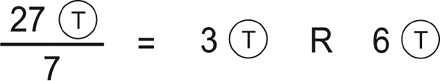
Let’s start by revisiting our earlier coin division of , this time using a new format:

 

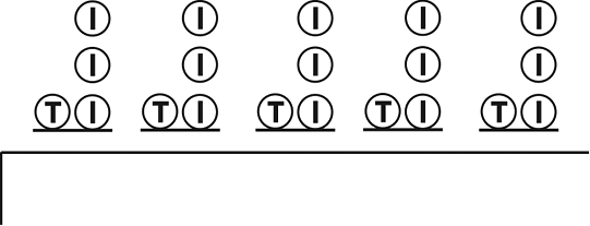
I.

 

 

 

The five slots above the bar have replaced the numeral 5.

 

II. Organize the s into groups of five:

 

 

 

III. Dealing the s into the five slots gives:

 

 

 

IV. Convert the remaining into s and arrange into groups of five:

 

 

 

V. Dealing the s into the five slots gives:

 

 

 

VI. Each portion size is , which gives as before:

 

= 13.

 

Let’s now see how the above process translates to numerical coefficient language:

 

• We first replace by

 

 

 

• For II and III, the process becomes divide 6 by 5 (this gives where,

 

):

 

 

 

• For IV, the process becomes

 

 

 

• For V, we have that and the process translates to:

 

 

 

• Thus we have that = 1 3 = 13.

 

Let’s next revisit using this new format:

 

I.

 

 

 

II. Divide the 3 s by 6 (this gives 0 R 3 ).

 

 

 

III. Convert the 3 s in the remainder to s :

 

 

 

IV. Divide the 34 s by 6 (this gives 5 R 4 ):

 

 

 

V. Convert the 4 s in the remainder into s:

 

 

 

VI. Divide the 48 s by 6 (this gives 8 R 0 ):

 

 

 

VII. Thus we have that = 5 8 = 58.

 

Note that since none of the steps in these procedures are marked out, it is possible for all of the steps I–VI to be condensed into one diagram.

We show how this is done with the division :

 

I.

 

 

 

II. Using a single diagram to perform all of the divisions (progressing from left to right), we obtain:

 

 

 

III. Thus we have that = 4 3 6 or 436.

IV. As with multiplication on diagrams, alignments abound. In II, if we simply drop the coins on the remainder values when we move them up, we further abbreviate things with no loss of information:

 

 

 

The content of the modern LDA is contained in these coin/coefficient methods. To reach the final stage in this play simply requires that we vertically stack the horizontal steps and jettison the coins.

Long Division with HA Numerals

To show how we get the LDA from the prior situation, we will reorganize the last division . Instead of pushing the remainders up and to the right as we progress through the division, we can just as conveniently push the numerals in the dividend down and to the left like so:

 

 

 

This can be shortened to:

 

 

 

Magic happens now if we jettison the coins and bring the numerals closer together:

 

 

 

This is the modern LDA, where we have explicitly shown the step involving the lead zero. In practice, this is usually left off. In comparing this diagram with the previous one, we clearly see that the change in coin denominations in the hybrid division algorithm translates to vertical steps in the LDA.

We make this explicit in the division of by labeling the various steps:

 

 

 

The answer to this division is 567 and it naturally and quite swiftly gives the answer to any of the following questions:

 

• How many times can we subtract 12 from 6804?

• How many groups containing 12 objects can we form out of 6804 objects?

• What are the portion sizes if we take 6804 objects and distribute them equally into 12 slots?

 

Each of these questions can of course take on an infinite number of guises including:

 

 

 

The LDA provides a systematic way of solving division problems. However, as we have already seen, it is not always the quickest way to divide. In many cases, we may do the division faster by canceling out trailing zeros or by simply knowing what number works in one fell swoop (as we did many times in chapter 8).

Even when long division is required it is not always necessary to use every step. For instance, we generally leapfrog the first steps if they yield leading zeros. For example in the prior division, we would generally make a mental note that 12 doesn’t go into 6 and immediately go to work on the next step of finding out how many times 12 goes into 68. In this case, our writing of the quotient would not include the lead zero. We may also skip steps by making even bolder guesses (e.g., instead of guessing how many times 12 goes into 68 we might be more daring and try to guess how many times 12 goes into 680). These are luxuries afforded to us in HA form that are not as available to us when we divide with coin numerals (or even to some extent using numerical coefficients)—demonstrating yet again how HA numerals are truly the Cadillac of all of the numeral systems discussed in this book.

The Great Division

In comparison with our methods for adding, subtracting, and multiplying in HA script, the LDA is a relative newcomer. Prior to 1500, the most common method of dividing with HA numerals was radically different from the LDA. It was known as the galley or scratch method.3 The following figure shows the method at work in dividing 73,485 by 214:

 

 

Before Dividing After Dividing

 

The quotient is the number to the right of the bar and the remainder consists of the “unscratched” out numerals on the left side of the bar (reading from left to right). This gives an answer of 343 remainder 83. Don’t worry if it looks confusing—it should if you never saw it before. But since the numerals sprout out somewhat evenly around the original diagram as opposed to expanding vertically down from it, the galley method actually takes up less space than the LDA. We won’t give the details on how the method works here; to do it justice would take us too far afield. Also, in practice, the numerals were not always scratched out.

The name galley was given to this division because its outline was thought by many to bear a resemblance to the galley ships which dominated the Mediterranean for more than 2,000 years.4 A particularly ornate example of the division was given in the unpublished Opus Arithmetica, a work attributed to a Venetian monk dating back to the sixteenth century:

 

 

Opus Arithmetica of Honoratus: Mathematical Treasures5

Image is from unpublished sixteenth-century manuscript (Opus Arithmetica of Honoratus: Mathematical Treasures). Footnote 5 has more information. Image is in the public domain.

 

If we so wished, we could adorn our own galley division above like so:

 

 

 

Some teachers in Venice, evidently, made it a requirement that students embellish their galley divisions with such designs.6

The galley technique eventually gave way in the 1500s to the method of division called “a danda” (the method which gives). Called “the great division” by one Italian writer of the time, it is in essence the LDA we currently use. The word “gives” was used because the procedure involves giving a new numeral to each remainder before starting the next division. In its early form, a danda involved placing the quotient on the right as in the galley method but over time the method evolved to a current form in some countries of placing the quotient on the top. This was most likely a result of the arrival in the late 1500s of the decimal notation for fractions which in some renditions of a danda required divisions to grow to the right (as more zeros were added after the decimal point) which would lead to interference if the quotient remained on the right.

Most historians in the nineteenth and early twentieth century thought that the galley method originated in ancient India but Lam Lay Yong of Singapore has made a strong case indicating that, while certainly practiced in India in the early centuries CE, use of the technique in China most likely predates this.7 The origins of our LDA are unknown. It made its first known appearance in print in 1491 in a work by Philipi Calanderi. As controversial among educators as the algorithm is today, it has the peculiar distinction of totally annihilating its chief sixteenth-century rival (although this took some time). For all intents and purposes, the galley method of division is now obsolete. None of the major algorithms for the other three operations that were in place during the sixteenth century can make such a claim.8 Of the rival methods that exist today for adding, subtracting, and multiplying numbers, many of them were also rivals with each other in the 1500s as well.

Conclusion

Thus concludes our directed study on the conceptual workings of the four elementary operations of arithmetic. Three of them yield to automatic handling once the tables and algorithms have been mastered, with the fourth, division, being effectively tamed with an intelligent guess or two, when needed, to get and keep the LDA rolling.

Division is not the last of the operations of arithmetic, however. Higher order operations, known as exponentiation (or raising to powers) and its inverse known as the taking of roots (e.g., the square or cube root), also exist.

The taking of exponents corresponds to repeated multiplication (when dealing with whole numbers). Thus, if we multiplied 6 × 6 × 6 × 6, we would abbreviate it as 64. The number 6 is called the base (the number being repeatedly multiplied) while the 4 is called the exponent (the number of times we involve the base in the multiplication). If we had 815, this would mean multiply fifteen eights together.

Can we domesticate repeated multiplication in the same manner as we have the four elementary operations? At the present time, the answer appears to be in the negative, as no simple written grade school algorithms, other than simply performing all of the multiplications, seems achievable. A procedure in writing that allows us to circumvent the repeated multiplications does exist, but it is too sophisticated and messy for the elementary school. Historically, it required the construction of an intricate table that proved exhausting to develop. The Scotsman John Napier, for example, spent nearly two decades of his life, in the late sixteenth and early seventeenth centuries, working on such a table. The logarithms he developed, and that were subsequently improved upon, form the centerpiece in this algorithm. Their use extended and greatly simplified not only the taking of exponents and roots but also the very large and messy multiplications and divisions involving decimals that scientists, such as the astronomer Johannes Kepler, were beginning to encounter.

Surprisingly, logarithms quickly allowed for the creation of a physical device that would far outdistance the abacus in its ability to perform sophisticated computations. Reaching a mature form by the middle of the seventeenth century, the slide rule is a device that can mechanically represent calculations with logarithms in an analogous way that the abacus is a device that mechanically mimics calculations in positional systems. Interestingly, in the case of the abacus, the device preceded the script (HA numerals), while in the case of the slide rule, the script (logarithms) preceded the device.

The question as to who actually invented the slide rule has been somewhat disputed—with the names of Englishmen William Oughtred, Richard Delamain, Edmund Gunter, and Edmund Wingate figuring prominently in the debate. An extremely valuable tool, the slide rule saw its heyday end only relatively recently in the late 1960s and early 1970s with the advent of electronic calculators—but that’s a whole other story.

Our approach to arithmetic so far has hopefully demonstrated that mathematics doesn’t sit alone in a vacuum, and that its symbols take their forms, in part, based on the needs and limitations of the human beings who developed them. As Raymond Wilder states, “Mathematics was born and nurtured in a cultural environment. Without the perspective which the cultural background affords, a proper appreciation of the context and state of present-day mathematics is hardly possible.”9

This is true not only of mathematics proper but also of the manner in which mathematics is explained to others. In fact, mathematics education forms its own complex and fascinating subplot in the two vast dramas that comprise its name—mathematics itself and education. Both subjects have rich histories of their own and remain of immense importance today. The same is no less true of their spectacular convergence. It is to this fascinating and important story that we next direct our attention.