Long-Term Change of Happiness in Nations
Two Times More Rise Than Decline Since the 1970s
Ruut Veenhoven, Erasmus University Rotterdam, The Netherlands; North-West University, Potchefstroom, South Africa
Several theories of happiness hold that happiness will not change in the long run. This claim was tested using the time trend data available in the World Database of Happiness. Series of responses on identical survey questions on happiness were selected with intervals of at least 10 years between them, altogether 199 time series in 67 nations and 1,531 data points. Average happiness in a nation rose in 133 of these series and declined in 66. The ratio of 2.0 is statistically significant. The average yearly rise in happiness on a scale 0–10 is +0.016. At this growth rate, happiness will rise by about 1 point on this scale in 70 years.
Keywords
happiness; life satisfaction; social progress; trend analysis; research synthesis
Introduction
Pursuit of Greater Happiness
Achieving happiness is a major goal in present-day Western society. Individually, people try to shape their lives in such a way that they can enjoy themselves. Politically, there is support for policies that aim at greater happiness for everybody. It is widely believed that we can get happier than we are, and there is also consensus that we should not acquiesce to current unhappiness.
The belief that we can get happier is rooted in the Enlightened view of man. Rather than a helpless being expelled from Paradise, man is seen as autonomous and able to improve his condition through the use of reason. This view was at the core of the 19th century Utopian movement and is still at the ideological basis of the 21th century welfare states. Planned social reform guided by scientific research is expected to result in a better society with happier citizens.
The conviction that we should try to improve happiness is also rooted in Enlightened thought. The notion that happiness is to be preferred above unhappiness can be found in the ancient Greek moral philosophy, such as in Epicurism. In the 18th century, it crystallized into the Utilitarian doctrine that the moral value of all action depends on the degree to which it contributes to the “greatest happiness for the greatest number” (Bentham, 1789). Although few accept happiness as the only and ultimate goal in life, it is generally agreed that happiness is a worthwhile goal. Happiness ranks high in public opinion surveys on value priorities. See, for example, Harding (1985, p. 231) and Diener and Oishi (2004).
This ideology is not unchallenged, however. It is argued that happiness is not the most valuable goal, and it is claimed that we cannot get happier even if we would want to. In this chapter, I focus on that latter objection.
Claim That Greater Happiness Is Not Attainable
The objection that we cannot raise happiness rests on two lines of thought. The first is that we are unable to create better living conditions. The second denunciation is that even a successful improvement in living conditions would help little because happiness tends to remain at the same level.
Life Not Getting Better
Enlightened progress optimism has been disputed on several grounds. One is the idea of a misfit between recent societal development and human nature. Critics of modernization see growing loneliness and alienation and assume that life was better in the good old days (e.g., Easterbrook, 2003). A related view holds that we are unable to create a more livable society and that attempts at social engineering have brought us out of the frying pan into the fire. In this view, happiness is declining rather than rising, and this is seen to manifest in soaring rates of suicide and depression. The idea that life was better in the past is also rooted in public opinion (Hagerty, 2003).
Happiness Not Responsive
Next, there are psychological theories that hold that an improvement in living conditions will not result in greater satisfaction with life.
Comparison theory
One such theory is that our assessment of happiness results from a comparison of life as it is and standards of how life should be, and that happiness is therefore “relative.” Any improvement in living conditions would soon result in a rise in our standards of comparison and would therefore leave us as (un)happy as before. In this theory, the pursuit of happiness will lead us on to a hedonic treadmill (Brickman & Campbell, 1971).
This theory also predicts that average happiness in nations will tend to the neutral—that is, around 5 on a scale of 0 to 10. Because we compare what we have with what compatriots have, there will always be people who do better or worse, irrespective of the level of living in the country.
Trait theory
The other theory is that happiness is a fixed “trait” rather than a variable “state.” Improvements of external living conditions will therefore not result in greater happiness, our evaluation of life being largely determined by an internal disposition to enjoy it or not. This theory has several variants.
One is set point theory, which holds that humans are hard-wired to maintain a similar degree of happiness—that is, a level 7 or 8 on scale of 0 to 10. In this view, happiness is maintained homeostatically and is, as such, comparable to body temperature. Cummins (1995) is a proponent of this view.
Another variant holds that there are inborn differences in our aptness to be happy or not. In this view, happiness is a temperamental disposition, possibly based in the neuro-physiological structure of pleasure centers in the brain. Some people are apt to feel cheerful and hence be positive about their life, even in difficult conditions, whereas others are prone to depression and hence judge their lives negatively even in favorable situations. See, for example, Lykken (1999).
Another variation is that happiness is an acquired disposition. Some people will develop a positive attitude toward life, whereas others will become sour. In this vein, Lieberman (1970, p. 74) wrote “… at some point in life, before even the age of 18, an individual becomes geared to a certain stable level of satisfaction, which—within a rather broad range of environmental circumstances—he maintains throughout life.”
Sociologists taking this perspective see the happiness of individuals as a reflection of collective national character. The outlook on life implied in common values and beliefs is seen to pervade individual perceptions and evaluations. Because collective outlook is largely an invariant matter, individual judgments geared by it are also seen to be rather static.
Easterlin Paradox
All these theories about unresponsive happiness figure in explanations for the Easterlin Paradox, which holds that average happiness in nations has not risen during the past decade in spite of impressive economic growth (Easterlin 1974, 1995, 2005; Easterlin, Aggelescu-McVey, Switek, Sawangfa, & Smith-Zweig, 2010).
Earlier Research
The idea of unresponsive happiness dates from the 1970s, when data about happiness in nations were scarce. Evidence for this theory crumbled when more data became available.
Comparisons of happiness across contemporary nations reveal large differences, such as an average, on a scale of 0 to 10, of 8.3 in Denmark and only 2.7 in Togo. See Veenhoven (2013a) for an overview of average happiness in 146 nations over the years 2000–2009. Most of the averages are far beyond the neutral 5 predicted by comparison theory, and about half of the scores are outside the range of between 7 to 8 predicted by set point theory.
Correlational analysis reveals strong associations between average happiness and several nation characteristics, such as economic development, freedom of the press, and rule of law. Abundant data on that topic are gathered in the report “Happiness and Conditions in the Nation” of the World Database of Happiness (Veenhoven, 2013b). This contradicts the idea that happiness is unresponsive to living conditions in the country.
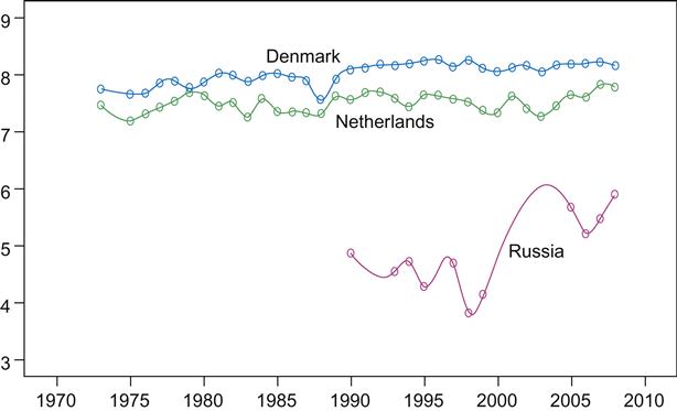
Comparison of happiness over time has further shown that average happiness has risen in some countries and declined in others. An example of gradually rising happiness is Denmark, where the average on a scale 0–10 rose from 7.6 in 1973 to 8.3 in 2012. Examples of declining happiness are found in Russia after the ruble crisis of the late 1990s and in Greece since the economic recession of 2010. These illustrative time trends are presented in Figure 9.1. More such trend data are available in the “Trend Report of Average Happiness” generated from the World Database of Happiness (Veenhoven, 2013c). These data leave no doubt that happiness can change and that happiness is responsive to changes in living conditions within an individual’s country.
Research Questions
So the question is not whether average happiness in nations can change, but how often has it changed and to what degree? Answering these questions is a first step to identifying the societal conditions that are most crucial to happiness and to feeding the political process with this information.
Happiness
The answers to the preceding questions depend on the precise concept of happiness used. Some things called happiness are more static than others. “Eudaimonic” happiness is, for instance, likely to be more stable than “hedonic” happiness, because the former concept denotes a set of personality traits, whereas the latter refers to a variable state of appreciation of life.
Concept
In this chapter, I focus on the latter kind of happiness—hedonic happiness. Happiness is defined as the degree to which an individual evaluates the overall quality of his or her life as a whole positively. This definition is delineated in more detail in Veenhoven (1984, ch. 2). This concept is in line with the Utilitarian notion of happiness as the “sum of pleasures and pains.” A synonym is “life satisfaction.”
Measures
Happiness as defined here can be measured using questions. Various claims to the contrary have been disproven empirically (research reviewed in Veenhoven, 1984, ch. 3). Although happiness is measurable in principle, not all the questions and scales that are used to measure this kind of happiness are valid. Elsewhere, I have reviewed current indicators and distinguished between those that are acceptable and those that are not (Veenhoven, 1984, ch. 4). In this chapter, I consider only data based on indicators that are deemed acceptable. As a consequence, several well-known studies on this matter have been left out. The studies on which this chapter is based were located using the World Database of Happiness (Veenhoven, 2013).
Long-term change
The above-mentioned theories of stable happiness do allow for short-term fluctuations. Comparison theory assumes that meeting aspirations will boost happiness temporarily until this advancement is neutralized by rising aspirations. Likewise, trait theories hold that happiness may vary somewhat with ups and downs in life: a trait happy person will be relatively happy in the year of marriage and unhappy in the year the couple divorces, but in the long run this person will oscillate around the same happiness level. Although such individual variations will balance out in the population of a nation, collective happenings may still affect the average—for instance, an economic recession or threat of war. For this reason, I consider only long-term changes in average happiness in nations, that is, for periods of at least 10 years.
Data
The data on average happiness in nations were taken from the World Database of Happiness (Veenhoven, 2013). This is a “findings archive” on happiness in the sense of subjective enjoyment of one’s life as a whole.
World Database of Happiness
The archive contains research findings yielded with measures that fit this concept of happiness as life satisfaction. All acceptable indicators are included in the collection “Measures of Happiness” (Veenhoven, 2013e).
Most measures are single survey questions, such as the famous item “Taking all together, how happy would you say you are these days; are you very happy, pretty happy, or not too happy?” This is just one of many acceptable measures of happiness. Survey questions have used different keywords, such as “satisfaction with life,” and different response options, such as numerical scales. Next to these single questions, there are also multiple questions, some of which constitute a “balance scale.”
This diversity of the measures of happiness used in the many surveys makes it difficult to compare scores and, in particular, to assess change in average happiness over time. The different measures of happiness have therefore been sorted into “equivalent” kinds—that is, questions that address happiness using the same keyword and a rating scale of the same length.
Research findings yielded using these acceptable measures of happiness are described in standard excerpts using standard terminology. Two kinds of findings are distinguished: distributional findings and correlational findings. Distributional findings denote how happy people are in a particular population and are often summarized in a measure of central tendency, typically the mean. Correlational findings are about things that go together with more or less happiness and summarized using measures of association, such as Pearson’s correlation coefficient.
Distributional findings are sorted into findings among special publics, such as senior citizens, and findings in the general population. The findings on happiness in the general public are further subdivided by the kinds of areas from which samples were drawn, such as regions, cities, and nations. These latter findings are gathered in the collection of “Happiness in Nations” (Veenhoven, 2013d), which we used for this research.
Collection Happiness in Nations
To date (September 2013), the collection “Happiness in Nations” contains 6,539 findings on average happiness in 167 nations over the years 1946–2012. These findings are sorted in three levels: (1) by nation, (2) within nations by kind of measure used, and (3) within measures of the same kind by year.
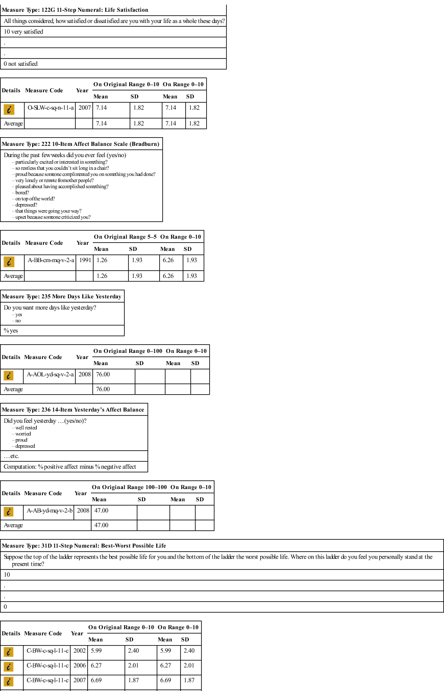
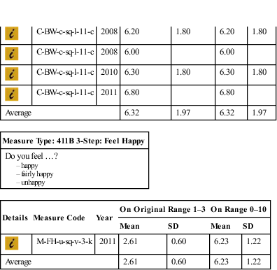
An example of a “nation page” is presented in Appendix 9.1. This is the case of Argentina for which 35 distributional findings are available. These findings are sorted in blocks of equivalent survey questions. The first block consists of seven findings yielded by a survey question on how “happy” one is, the answers to which are rated on a four-step verbal response scale. The measure codes link to the precise text of that specific question, and detailed information about the investigation can be found behind the “i” icon.
Findings are sorted by year within each block, and this first block consists of the years 1981, 1991, 1995, 1999, 2002, 2005, and 2008. Looking at the blocks in Appendix 9.1, we see no clear trend in the responses to the question on happiness (measure type 111c) between 1981 and 2008, but a gradual change to the better in the responses to questions about life satisfaction (measure type 121C and 122F) and the Cantril ladder (measure type 31D).
Identical Questions
Within these blocks of equivalent questions, there are still small differences in the wording of the lead question and/or response options. These variations are marked by the last symbol in the measure code. There are also variations in the time frame addressed in the question, and these are marked with the third letter code, where “c” stands for “current,” “g” stands for in “general,” and “u” is used for “unclear.” These minor variations in the wording of questions can result in small differences in the mean scores and could, as such, overshadow the small changes in actual happiness over time. Together with Floris Vergunst I selected a set of time series based on identical questions—that is, questions with the same measure code.1
In the above-mentioned case of seven questions on how “happy” one is in Argentina, this meant that we considered only the five findings based on the question variant “a.” Because the series of answers to question variant “f” covered only 6 years, they were left out.
Transformation to a Common 0–10 Numerical Scale
We used the transformed means, provided in the World Database of Happiness, for reasons of comparability. These transformed means are expressed on a common numerical scale ranging from 0 (low) to 10 (high). Scores on numerical response scales, shorter than this, are linearly stretched to give a range of 0–10. Scores on scales with verbal response options are transformed using a procedure first described by Thurstone (1927), in which experts rate the numerical value of response options. This procedure is described in more detail in Veenhoven (1993, ch. 7).
Series
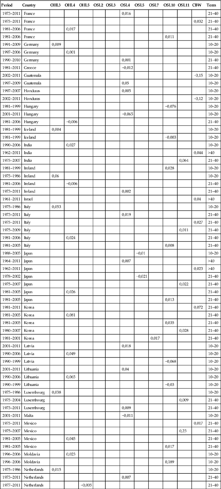
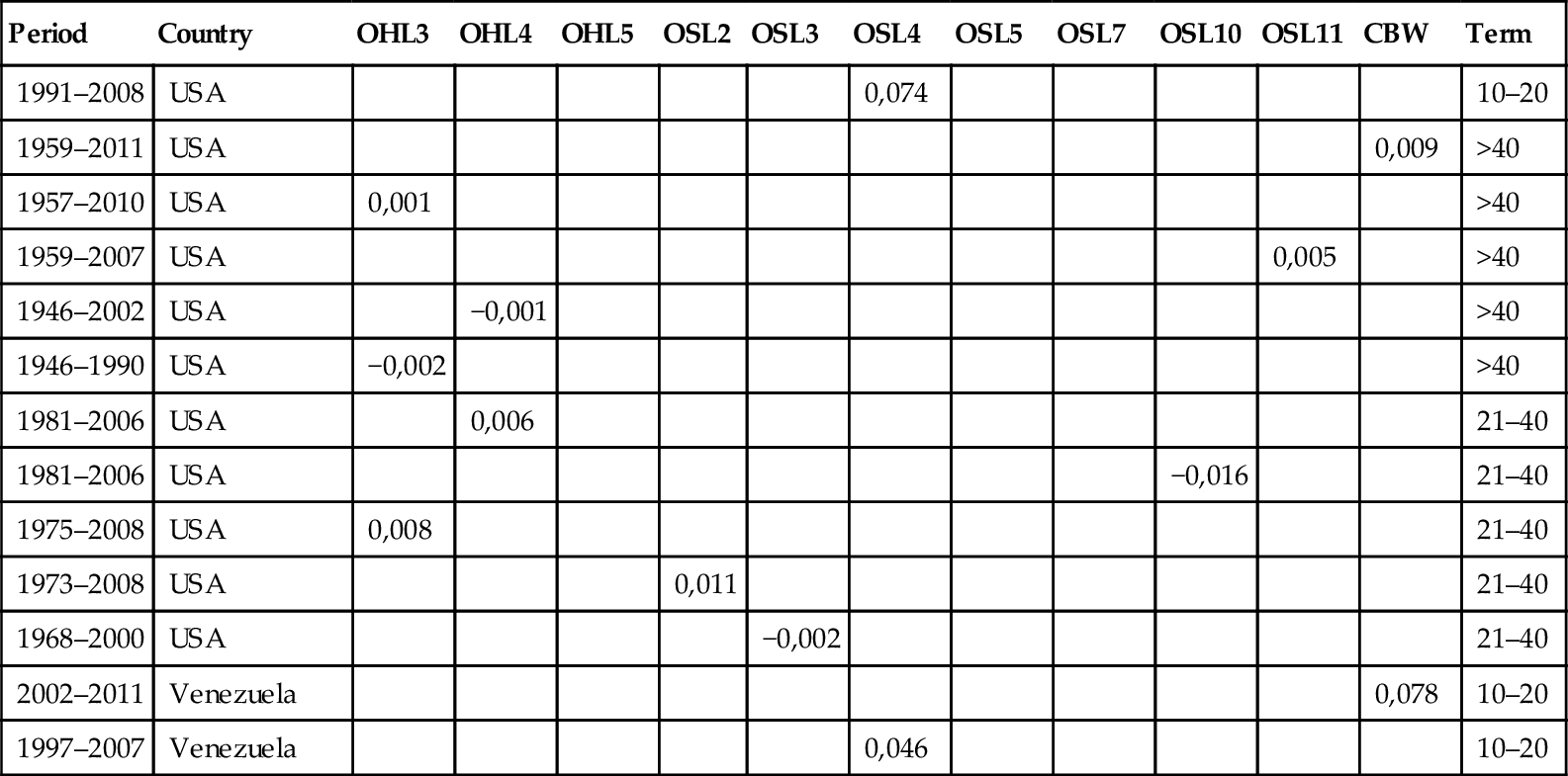
On this basis, several series of responses to identical questions on happiness in the same nation over time were constructed. We limited our analysis to series that covered a minimum of 10 years. We also limited the analysis to data gathered using probability samples. If the same question was used in several surveys in the same year in the same country, we used the average response to that question. We did not require that a series contain more than two data points, although most series had more. This resulted in 199 time series for average happiness in 67 nations, which together gave 1,531 data points. The data matrix is presented in Appendix 9.2. This work was done in the context of a test of the Easterlin Paradox (Veenhoven & Vergunst, 2014).
From the data discussed above, we selected series that involved at least 30 data points over at least 20 years and that were sufficiently dense for a meaningful test of significance to be performed.
Method
The question is whether average happiness has typically remained at the same level in nations, or has it risen in most nations?
One way to answer this question is to consider the effect size and pick a minimum, such as over a 10-year period, a 0.1 point change in happiness. In this case, our conclusions are limited to the series studied here.
Another way is to generalize beyond the observations, and in this context, it is common practice to infer the probability that the change observed in the sample is positive, while there is actually no correlation in the population from which this sample is drawn. In this context, a 95% probability is usually deemed “significant.”
Although routinely performed, this test for significance involves making strong assumptions that do not fully apply in this case. One such assumption is that the 199 series provide a random sample of all possible time series in the 67 nations. Another dubious assumption is that the 67 nations provide a random sample of all nations in the world.
Still other points to keep in mind are that significance depends very much on the sample size, small effects are significant in big samples, and big effects are insignificant in small samples. In the time series at hand, the number of data points is typically too small for a meaningful test. Significance also depends on the dispersion in the observations and on choices made by the investigator, with respect to the null hypothesis, one-sided or two-sided testing, and the probability level. All this makes tests for significance precarious.
In my view, the descriptive approach is the most informative in this case. The number of series at hand is large and covers all we will ever be able to obtain for this period. The interpretation is straightforward; we can easily see in Appendix 9.2 where the Easterlin Paradox applies—coefficient 0—and where not—all the positive coefficients.
Still, I realize that many readers are accustomed to significance testing and some are willing to buy into the above-mentioned perils, even when acknowledged. I therefore did some significance tests. I tested whether the observed positive change in happiness was more common than negative change and whether the average change coefficient was significantly different from zero.
I also considered some sufficiently dense time series separately and assessed whether, in each of these cases, the linear change coefficient differed significantly from zero. In this case, the test informs us about the probability that the observed trend in this series mirrors the trend in the general population—in other words, of the probability that another sample of surveys in the same country over the same years would yield the same results.
Change in All 199 Series
I regressed happiness against year in all the 199 time series. The resulting regression coefficients were used to indicate the yearly change in happiness in the period covered by the series. Because happiness is expressed on a scale of 0–10, a regression coefficient of 0.01 means a rise of 0.1 point per year, which amounts to a 1-point gain in happiness over 10 years. These yearly coefficients were used in the following ways.
Ratio of Rise or Decline
We first counted the number of series in which happiness had gone up and the number in which happiness had gone down. On that basis, I assessed the ratio: a ratio greater than 1 indicates that increasing happiness is more common than decline; a ratio of 1, that rising and declining happiness are equally frequent; and a ratio smaller than 1, that a decline in happiness is the most common. The theory of stable happiness predicts a ratio of 1. Deviation from that level was tested for significance.
Average Change Coefficient
The above bipartitions provide a view on the relative frequency of rise and decline in happiness, but do so at the cost of loss of variation. To use the available variance more fully, I computed the average change over all 199 series and assessed whether that average coefficient was positive or negative. I next tested whether the difference from zero was statistically significant.
Grouping by Country
Using the change coefficients in the series, we computed the average change coefficients for each of the 67 nations. Where only one series was available, I took the change coefficient observed in that one, and when more series were available, I computed the average change score.
These change scores in nations were analyzed in the same way as the change scores in the series. First, a ratio of rise or decline in happiness was obtained; then the average change scores were computed and we assessed the statistical significance of these scores.
Significance 18 Dense Series
Following standard practice in the World Database of Happiness, we selected time series of at least 30 data points over a period of at least 20 years. Together, 18 such series are available: one for each of the 10 EU nations where the Eurobarometer surveys started in the 1970s; one for Japan since 1958; and three for the United States, where different series were started in the 1950s. A coefficient of linear change was computed for each of these series, and the statistical significance of that coefficient was tested at the 55 level.
Results: More Advance than Decline in All Series
Ratio of Rise and Decline
Of the 199 series, 66% showed a rise in happiness and 34% a decline, which resulted in a ratio of 1.9. Likewise, happiness rose in 64% of the 67 nations and declined in 36%, which is a ratio of 1.6. See Table 9.1. This is clearly more than the ratio of about 1 predicted by the theory of stable happiness.
Table 9.1
Change of Average Happiness in 67 Nationsa
Frequency of rise versus decline over periods of at least 10 years
| Pattern of Change | Series | Nations | ||
| N | % | N | % | |
| Rise | 133 | 66% | 42 | 62% |
| Decline | 66 | 34% | 25 | 38% |
| Total | 199 | 100% | 67 | 100% |
| Ratio rise-decline | 1.94 | 1.64 | ||
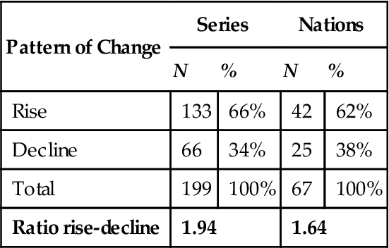
aSource: Veenhoven (2013d).
Average Change Coefficients
The average yearly rise in happiness observed in the 199 series is +0.016. The average rise in the 67 nations was +0.012.
These numbers may seem small at first sight but result in a considerable improvement in happiness in the long term. At this growth rate, average happiness will rise 1 point on a 0–10 scale in 70 years. Given that the actual range on this scale is between 2.5 and 8.5 (Veenhoven, 2012a), a 1-point rise equals a gain of 17%.
Similar Across Time Spans
In their latest paper, Veenhoven and Vergunst (2014) argued that happiness rises only in the short term. The data show otherwise. We can see from Table 9.2 that the average change in happiness does not differ very much between the short and the long term and that the rise is slightly stronger in the long term.
Table 9.2
Change of Average Happiness in Nationsa
Average yearly change in points on scale 0–10, split up by length of period
| Period | Series | Nations | ||
| N | b | N | b | |
| Short term | 114 | +0.017 | 31 | +0.010 |
| Medium term | 67 | +0.013 | 27 | +0.009 |
| Long term | 18 | +0.020 | 9 | +0.030 |
| Total | 199 | +0.016 | 67 | +0.012 |
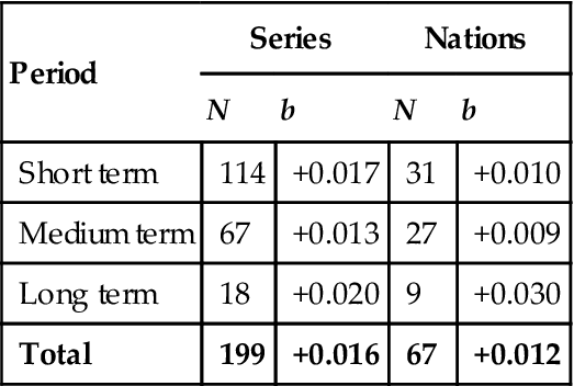
aSource: Veenhoven and Vergunst (2014).
Significant in Most of the Dense Series
The changes in happiness observed in series consisting of 30 or more data points over at least 20 years are presented in Table 9.3. The last column presents the change in points on a 0–10 scale. The bold printed changes are significantly different from zero. As one can see, the changes range between a gain of more than half a point in the case of Italy and a similar loss in the case of Portugal. The observed change is significantly different from zero in 11 of these cases and insignificant in 6 cases.
Table 9.3
Change of Average Happiness in 14 Nationsa
Time series of at least 30 observations over at least 20 years
| Nation | Question | Years | Data Points | Change in Average Happiness on Scale 0–10 | ||
| Average Yearly Change | Total Change in Points | |||||
| Change Coefficient | 95% Significance Interval | |||||
| Belgium | O-SLL-u-sq-v-4-b | 1973–2012 | 70 | −.007 | −.016 to +.002 | −0.27 |
| Denmark | O-SLL-u-sq-v-4-b | 1973–2012 | 69 | +.015 | +.011 to +.018 | +0.59 |
| France | O-SLL-u-sq-v-4-b | 1973–2012 | 69 | +.016 | +.011 to +.021 | +0.62 |
| Germany (West) | O-SLL-u-sq-v-4-b | 1973–2009 | 65 | +.000 | −.007 to +.007 | 0.00 |
| Greece | O-SLL-u-sq-v-4-b | 1981–2012 | 58 | –.021 | −.036 to −.006 | –0.67 |
| Ireland | O-SLL-u-sq-v-4-b | 1973–2012 | 69 | +.002 | −.006 to +.009 | +0.08 |
| Italy | O-SLL-u-sq-v-4-b | 1973–2012 | 69 | +.012 | +.004 to +.020 | +0.47 |
| Japan | O-SLu-c-sq-v-4-e | 1964–2013 | 49 | +.004 | +.000 to +.008 | +.20 |
| Luxembourg | O-SLL-u-sq-v-4-b | 1973–2012 | 69 | +.009 | +.005 to +.014 | +0.35 |
| Netherlands | O-SLL-u-sq-v-4-b | 1973–2012 | 69 | +.008 | +.003 to +.012 | +0.31 |
| O-HP-u-sq-v-5-a | 1977–2011 | 57 | −.001 | −.003 to +.000 | −0.06 | |
| Portugal | O-SLL-u-sq-v-4-b | 1985–2012 | 49 | –.035 | −.048 to –.021 | −0.98 |
| Spain | O-SLL-u-sq-v-4-b | 1985–2012 | 49 | +.011 | −.011 to +.016 | +0.31 |
| UK | O-SLL-u-sq-v-4-b | 1973–2012 | 68 | +.008 | +.005 to +.012 | +0.31 |
| USA | O-HL-c-sq-v-3-aa | 1974–2008 | 62 | +.009 | +.002 to +.016 | +0.29 |
| O-SLP-g-sq-v-2b | 1973–2008 | 45 | +.011 | +.005 to +.017 | +0.35 | |
| O-BW-c-sq-l-11a | 1959–2007 | 60 | +.013 | +.006 to +.020 | +0.62 | |

aSource: Veenhoven (2013c).
Happiness has remained almost stable in the case of West Germany, which is at least partly due to the influx of many unhappy East Germans after reunification in 1990. In the other cases, statistical insignificance does not denote that happiness has not changed. Happiness has gone up and down in Belgium and Greece, and these bumps are not reflected in the coefficient of linear change. Inspection of trend plots shows greater variation in yearly scores for Japan and the United States, probably due to smaller sample sizes and slight differences in the wording of questions and their place in the questionnaire. As noted previously, significance depends also on the dispersion of observations.
Discussion
The data presented here leave us with no doubt that happiness in nations can change; average happiness has changed in most countries for which we have data since the 1970s, and typically to the positive. This begs the question of why so many came to believe that happiness is immutable. Another question is how well the observed change in average happiness fits with trends in other aspects of human thriving.
Why the Belief in Stable Happiness in Nations
One answer to this question about change in happiness lies in data availability. This theory emerged in the 1970s when the differences across countries were more apparent than the change within countries over time. Time series were scarce in those days and too short to capture the small increments in happiness. The view on change in happiness was also blurred by imperfections in the first available time series. The most prominent series is a series of responses to a question on happiness rated on a three-step scale in the United States, which has shown no rise since the first assessment made in 1945. Yet this series started in the euphoric time of a war won, and the wording of the questions differed slightly until 1972. Identical questions used since 1973 do show a slight rise in average happiness, as shown in Table 9.3. Likewise, changes in the wording of survey questions in Japan have veiled a trend to the positive since 1958, as shown by Suzuki (2009).
Another reason for the belief that happiness is immutable lies in data analysis and, in particular, in the interpretation of tests of significance of changes in happiness. Absence of significance is taken as proof of stability, instead of being seen as a lack of statistical power. Remember the earlier “Method” section, in which I argued that most of the time data series on happiness do not meet the requirements for a meaningful significance test.
A third reason lies in the theory of happiness. Happiness is commonly seen to result from a cognitive comparison between what one wants and what one has, and in that view a hedonic treadmill is plausible. The theory that happiness depends on the gratification of needs in the first place has less appeal, in particular among sociologists, although it fits better with the facts (Veenhoven, 2008). Likewise, psychologists tend to focus on stable traits rather than on variable states, and for this reason the stability of happiness is more prominent in their perspective.
Still another reason lies in ideology. The belief that happiness does not rise in spite of economic growth fits well with several strands of social criticism, such as criticism of capitalism, globalization, mass consumption, and environmental degradation. Activists spread this belief to promote their cause, actively using all the media available.
Related Trends in Living Conditions
Material living conditions have improved in most countries since the 1970s, and this gain is reflected in rising GNP per capita. Contrary to the earlier mentioned Easterlin Paradox, there is a clear relation with happiness. The greatest rise in happiness is observed in the countries where the economy has grown the most: r=+0.22 (Veenhoven & Vergunst, 2014). The recent economic recession has caused a considerable drop in average happiness in the most affected European countries: Greece, Spain, and Portugal.
There are also strong indications of lessening social inequality in developed nations. Although income differences have grown, differences in happiness have lessened, and inequality in happiness among citizens reflects the total effects of inequalities in all life domains. Inequality of happiness can be measured using the standard deviation. This appears in a comparison of standard deviations of happiness over time (Kalmijn & Veenhoven, 2005). Standard deviations of happiness have shrunk in most nations since the 1970s, partly due to a reduction in the percentage of very unhappy people (Veenhoven, 2005a). So the rise in average happiness is typically accompanied with a reduction in differences among citizens.
Related Trends in Human Flourishing
Human flourishing is reflected in good health and finally in longevity. Life expectancy has also increased in most countries over the period considered here, and together with the observed rise in average happiness, this has resulted in a spectacular rise in “Happy Life Years” (Veenhoven, 2005b), which is paralleled by a similar rise in years lived in good health. Life is getting better, and the rise of average happiness in nations is just one indicator of that development.
Conclusion
Average happiness in nations has changed in most nations over the past decade and in most cases for the positive. Stable happiness in nations is the exception rather than the rule.
Appendix 9.1 Example of a Presentation of Findings on Average Happiness in Nations2
Table A9.1
Distributional Findings on Happiness in Argentina (AR)a
| Measure Type: 111C 4-Step Verbal: Happiness |
| Taking all things together, would you say you are: |
| very=4 … not at all=1 |
| Details | Measure Code | Year | On Original Range 1–4 | On Range 0–10 | ||
| Mean | SD | Mean | SD | |||
 |
O-HL-u-sq-v-4-a | 1981 | 2.95 | 0.65 | 6.80 | 1.88 |
|
O-HL-u-sq-v-4-a | 1991 | 3.07 | 0.82 | 7.00 | 2.27 |
|
O-HL-u-sq-v-4-a | 1995 | 3.09 | 0.73 | 7.13 | 2.01 |
|
O-HL-u-sq-v-4-a | 1999 | 3.13 | 0.75 | 7.20 | 2.08 |
|
O-HL-g-sq-v-4-f | 2002 | 2.60 | 0.92 | 5.11 | 2.64 |
|
O-HL-u-sq-v-4-a | 2005 | 3.20 | 0.67 | 7.45 | 1.78 |
|
O-HL-g-sq-v-4-f | 2008 | 3.03 | 0.72 | 6.37 | 2.03 |
| Average | 3.01 | 0.75 | 6.72 | 2.10 | ||
| Measure Type: 121C 4-Step Verbal: Life Satisfaction |
| How satisfied are you with the life you lead? |
| very=4 … not at all=1 |
| Details | Measure Code | Year | On Original Range 1–4 | On Range 0–10 | ||
| Mean | SD | Mean | SD | |||
|
O-SLu-g-sq-v-4-b | 1997 | 2.14 | 0.96 | 6.41 | 2.01 |
|
O-SLu-g-sq-v-4-b | 2000 | 2.21 | 1.01 | 6.52 | 2.02 |
|
O-SLu-g-sq-v-4-c | 2001 | 2.81 | 0.86 | 5.99 | 2.34 |
|
O-SLu-g-sq-v-4-c | 2003 | 2.91 | 0.77 | 6.27 | 2.13 |
|
O-SLu-g-sq-v-4-c | 2004 | 2.92 | 0.83 | 6.30 | 2.29 |
|
O-SLu-g-sq-v-4-c | 2005 | 2.92 | 0.84 | 6.30 | 2.31 |
|
O-SLu-g-sq-v-4-c | 2006 | 3.02 | 0.74 | 6.57 | 2.05 |
|
O-SLu-g-sq-v-4-c | 2007 | 2.85 | 0.75 | 6.11 | 2.04 |
|
O-SLu-g-sq-v-4-dc | 2008 | 3.01 | 0.77 | 6.82 | 2.00 |
|
O-SLu-g-sq-v-4-c | 2010 | ||||
|
O-SLu-g-sq-v-4-da | 2010 | 2.94 | 0.89 | 6.64 | 2.31 |
| Average | 2.77 | 0.84 | 6.39 | 2.15 | ||
| Measure Type: 122F 10-Step Numeral: Life Satisfaction |
| All things considered, how satisfied are you with your life as a whole now? |
| 10 satisfied |
| . |
| . |
| 1 dissatisfied |
| Details | Measure Code | Year | On Original Range 1–10 | On Range 0–10 | ||
| Mean | SD | Mean | SD | |||
|
O-SLW-c-sq-n-10-aa | 1981 | 6.80 | 2.10 | 6.44 | 2.34 |
|
O-SLW-c-sq-n-10-aa | 1990 | 7.25 | 2.03 | 6.95 | 2.25 |
|
O-SLW-c-sq-n-10-aa | 1995 | 6.92 | 2.32 | 6.58 | 2.58 |
|
O-SLW-c-sq-n-10-a | 1999 | 7.33 | 2.26 | 7.03 | 2.51 |
|
O-SLW-c-sq-n-10-a | 2006 | 7.79 | 1.91 | 7.54 | 2.12 |
| Average | 7.22 | 2.12 | 6.91 | 2.36 | ||
| Measure Type: 122G 11-Step Numeral: Life Satisfaction |
| All things considered, how satisfied or dissatisfied are you with your life as a whole these days? |
| 10 very satisfied |
| . |
| . |
| 0 not satisfied |
| Details | Measure Code | Year | On Original Range 0–10 | On Range 0–10 | ||
| Mean | SD | Mean | SD | |||
|
O-SLW-c-sq-n-11-a | 2007 | 7.14 | 1.82 | 7.14 | 1.82 |
| Average | 7.14 | 1.82 | 7.14 | 1.82 | ||
| Measure Type: 222 10-Item Affect Balance Scale (Bradburn) |
| During the past few weeks did you ever feel (yes/no) |
| Details | Measure Code | Year | On Original Range 5–5 | On Range 0–10 | ||
| Mean | SD | Mean | SD | |||
|
A-BB-cm-mq-v-2-a | 1991 | 1.26 | 1.93 | 6.26 | 1.93 |
| Average | 1.26 | 1.93 | 6.26 | 1.93 | ||
| Measure Type: 235 More Days Like Yesterday |
| Do you want more days like yesterday? |
| % yes |
| Details | Measure Code | Year | On Original Range 0–100 | On Range 0–10 | ||
| Mean | SD | Mean | SD | |||
|
A-AOL-yd-sq-v-2-a | 2008 | 76.00 | |||
| Average | 76.00 | |||||
| Measure Type: 236 14-Item Yesterday’s Affect Balance |
| Did you feel yesterday … (yes/no)? |
| … etc. |
| Computation: % positive affect minus % negative affect |
| Details | Measure Code | Year | On Original Range 100–100 | On Range 0–10 | ||
| Mean | SD | Mean | SD | |||
|
A-AB-yd-mq-v-2-b | 2008 | 47.00 | |||
| Average | 47.00 | |||||
| Measure Type: 31D 11-Step Numeral: Best-Worst Possible Life |
| Suppose the top of the ladder represents the best possible life for you and the bottom of the ladder the worst possible life. Where on this ladder do you feel you personally stand at the present time? |
| 10 |
| . |
| . |
| 0 |
| Details | Measure Code | Year | On Original Range 0–10 | On Range 0–10 | ||
| Mean | SD | Mean | SD | |||
|
C-BW-c-sq-l-11-c | 2002 | 5.99 | 2.40 | 5.99 | 2.40 |
|
C-BW-c-sq-l-11-c | 2006 | 6.27 | 2.01 | 6.27 | 2.01 |
|
C-BW-c-sq-l-11-c | 2007 | 6.69 | 1.87 | 6.69 | 1.87 |
|
C-BW-c-sq-l-11-c | 2008 | 6.20 | 1.80 | 6.20 | 1.80 |
|
C-BW-c-sq-l-11-c | 2008 | 6.00 | 6.00 | ||
|
C-BW-c-sq-l-11-c | 2010 | 6.30 | 1.80 | 6.30 | 1.80 |
|
C-BW-c-sq-l-11-c | 2011 | 6.80 | 6.80 | ||
| Average | 6.32 | 1.97 | 6.32 | 1.97 | ||
| Measure Type: 411B 3-Step: Feel Happy |
| Do you feel … ? |
| Details | Measure Code | Year | On Original Range 1–3 | On Range 0–10 | ||
| Mean | SD | Mean | SD | |||
|
M-FH-u-sq-v-3-k | 2011 | 2.61 | 0.60 | 6.23 | 1.22 |
| Average | 2.61 | 0.60 | 6.23 | 1.22 | ||

aSource: Veenhoven (2013d).
Appendix 9.2 Data Matrix
Table A9.2 a
| Period | Country | OHL3 | OHL4 | OHL5 | OSL2 | OSL3 | OSL4 | OSL5 | OSL7 | OSL10 | OSL11 | CBW | Term |
| 2002–2011 | Argentina | 0,078 | 10–20 | ||||||||||
| 1981–2005 | Argentina | 0,026 | 21–40 | ||||||||||
| 1981–2006 | Argentina | 0,039 | 21–40 | ||||||||||
| 1975–2008 | Australia | 0,011 | 21–40 | ||||||||||
| 1981–2005 | Australia | −0,005 | 21–40 | ||||||||||
| 1981–2005 | Australia | −0,001 | 21–40 | ||||||||||
| 1975–2011 | Australia | 21–40 | |||||||||||
| 1995–2011 | Austria | −0,027 | 10–20 | ||||||||||
| 1990–1999 | Austria | 0,187 | 10–20 | ||||||||||
| 1990–2006 | Austria | −0,029 | 10–20 | ||||||||||
| 1990–2000 | Belarus | 0,072 | 10–20 | ||||||||||
| 1990–2000 | Belarus | −0,09 | 10–20 | ||||||||||
| 1981–1999 | Belgium | 0,011 | 10–20 | ||||||||||
| 1989–2008 | Belgium | −0,032 | 10–20 | ||||||||||
| 1975–1986 | Belgium | −0,054 | 10–20 | ||||||||||
| 1973–2011 | Belgium | −0,008 | 21–40 | ||||||||||
| 1981–2006 | Belgium | 0,016 | 21–40 | ||||||||||
| 2002–2011 | Bolivia | 0,046 | 10–20 | ||||||||||
| 1997–2007 | Bolivia | −0,05 | 10–20 | ||||||||||
| 1990–2006 | Brazil | 0,054 | 10–20 | ||||||||||
| 1990–2006 | Brazil | 0,022 | 10–20 | ||||||||||
| 1960–2011 | Brazil | 0,046 | >40 | ||||||||||
| 2001–2011 | Bulgaria | 0,05 | 10–20 | ||||||||||
| 2002–2011 | Bulgaria | 0,021 | 10–20 | ||||||||||
| 1990–2006 | Bulgaria | 0,029 | 10–20 | ||||||||||
| 1990–2006 | Bulgaria | 0,019 | 10–20 | ||||||||||
| 1968–1977 | Canada | −0,009 | 10–20 | ||||||||||
| 1981–2000 | Canada | 0,01 | 10–20 | ||||||||||
| 1982–2000 | Canada | −0,004 | 10–20 | ||||||||||
| 1997–2010 | Chile | 0,009 | 10–20 | ||||||||||
| 1990–2005 | Chile | 0,017 | 10–20 | ||||||||||
| 1990–2005 | Chile | −0,025 | 10–20 | ||||||||||
| 1990–2007 | China | 0,002 | 10–20 | ||||||||||
| 1997–2011 | China | −0,005 | 10–20 | ||||||||||
| 1990–2009 | China | −0,019 | 10–20 | ||||||||||
| 1990–2010 | Costa Rica | −0,041 | 21–40 | ||||||||||
| 1995–2007 | Croatia | 0,019 | 10–20 | ||||||||||
| 1962–2011 | Croatia | 0,018 | >40 | ||||||||||
| 2001–2011 | Cyprus | 0,033 | 10–20 | ||||||||||
| 2001–2011 | Czech | 0,026 | 10–20 | ||||||||||
| 1990–2006 | Czech | 0,047 | 10–20 | ||||||||||
| 1981–1999 | Denmark | 0,003 | 10–20 | ||||||||||
| 1975–1986 | Denmark | −0,026 | 10–20 | ||||||||||
| 1972–2006 | Denmark | 0,019 | 21–40 | ||||||||||
| 1973–2011 | Denmark | 0,014 | 21–40 | ||||||||||
| 1962–2011 | Dom. Republic | 0,081 | >40 | ||||||||||
| 1997–2007 | Ecuador | −0,05 | 10–20 | ||||||||||
| 1960–2011 | Egypt | −0,012 | >40 | ||||||||||
| 1991–2010 | El Salvador | −0,04 | 10–20 | ||||||||||
| 1997–2006 | England | −0,006 | 10–20 | ||||||||||
| 1975–1986 | England | 0,023 | 10–20 | ||||||||||
| 1973–2011 | England | 0,008 | 21–40 | ||||||||||
| 1975–2011 | England | 0,002 | 21–40 | ||||||||||
| 1981–2006 | England | −0,002 | 21–40 | ||||||||||
| 1981–2006 | England | −0,003 | 21–40 | ||||||||||
| 1990–1999 | Estonia | −0,038 | 10–20 | ||||||||||
| 2001–2011 | Estonia | 0,091 | 10–20 | ||||||||||
| 1990–2006 | Estonia | 0,051 | 10–20 | ||||||||||
| 1956–2011 | Finland | 0,01 | >40 | ||||||||||
| 1972–2006 | Finland | 0,01 | 21–40 | ||||||||||
| 1981–2005 | Finland | 0 | 21–40 | ||||||||||
| 1975–1986 | France | −0,003 | 10–20 | ||||||||||
| 1973–2011 | France | 0,016 | 21–40 | ||||||||||
| 1975–2011 | France | 0,032 | 21–40 | ||||||||||
| 1981–2006 | France | 0,017 | 21–40 | ||||||||||
| 1981–2006 | France | 0,011 | 21–40 | ||||||||||
| 1991–2009 | Germany | 0,009 | 10–20 | ||||||||||
| 1997–2006 | Germany | 0,001 | 10–20 | ||||||||||
| 1990–2010 | Germany | 0,001 | 21–40 | ||||||||||
| 1981–2011 | Greece | −0,012 | 21–40 | ||||||||||
| 2002–2011 | Guatemala | −0,15 | 10–20 | ||||||||||
| 1997–2009 | Guatemala | 0,05 | 10–20 | ||||||||||
| 1997–2007 | Honduras | 0,005 | 10–20 | ||||||||||
| 2002–2011 | Honduras | −0,12 | 10–20 | ||||||||||
| 1981–1999 | Hungary | −0,076 | 10–20 | ||||||||||
| 2001–2011 | Hungary | −0,065 | 10–20 | ||||||||||
| 1981–2006 | Hungary | −0,006 | 21–40 | ||||||||||
| 1981–1999 | Iceland | 0,004 | 10–20 | ||||||||||
| 1981–1999 | Iceland | −0,003 | 10–20 | ||||||||||
| 1990–2006 | India | 0,027 | 10–20 | ||||||||||
| 1962–2011 | India | 0,044 | >40 | ||||||||||
| 1975–2007 | India | 0,064 | 21–40 | ||||||||||
| 1981–1999 | Ireland | 0,028 | 10–20 | ||||||||||
| 1975–1986 | Ireland | 0,06 | 10–20 | ||||||||||
| 1981–2006 | Ireland | −0,006 | 21–40 | ||||||||||
| 1973–2011 | Ireland | 0,002 | 21–40 | ||||||||||
| 1961–2011 | Israel | 0,04 | >40 | ||||||||||
| 1975–1986 | Italy | 0,053 | 10–20 | ||||||||||
| 1973–2011 | Italy | 0,019 | 21–40 | ||||||||||
| 1975–2011 | Italy | 0,027 | 21–40 | ||||||||||
| 1975–2009 | Italy | 0,011 | 21–40 | ||||||||||
| 1981–2006 | Italy | 0,024 | 21–40 | ||||||||||
| 1981–2005 | Italy | 0,008 | 21–40 | ||||||||||
| 1988–2005 | Japan | −0,01 | 10–20 | ||||||||||
| 1964–2011 | Japan | 0,007 | >40 | ||||||||||
| 1962–2011 | Japan | 0,023 | >40 | ||||||||||
| 1978–2002 | Japan | −0,021 | 21–40 | ||||||||||
| 1975–2007 | Japan | 0,022 | 21–40 | ||||||||||
| 1981–2005 | Japan | 0,026 | 21–40 | ||||||||||
| 1981–2005 | Japan | 0,013 | 21–40 | ||||||||||
| 1981–2011 | Korea | 0,072 | 21–40 | ||||||||||
| 1981–2005 | Korea | 0,081 | 21–40 | ||||||||||
| 1981–2005 | Korea | 0,035 | 21–40 | ||||||||||
| 1980–2007 | Korea | 0,028 | 21–40 | ||||||||||
| 1981–2001 | Korea | 0,017 | 21–40 | ||||||||||
| 2001–2011 | Latvia | 0,018 | 10–20 | ||||||||||
| 1990–2006 | Latvia | 0,049 | 10–20 | ||||||||||
| 1990–1999 | Latvia | −0,068 | 10–20 | ||||||||||
| 2001–2011 | Lithuania | 0,04 | 10–20 | ||||||||||
| 1990–2006 | Lithuania | 0,065 | 10–20 | ||||||||||
| 1990–1999 | Lithuania | −0,03 | 10–20 | ||||||||||
| 1975–1986 | Luxembourg | 0,038 | 10–20 | ||||||||||
| 1975–2004 | Luxembourg | 0,009 | 21–40 | ||||||||||
| 1973–2011 | Luxembourg | 0,009 | 21–40 | ||||||||||
| 2001–2011 | Malta | −0,011 | 10–20 | ||||||||||
| 1975–2011 | Mexico | 0,017 | 21–40 | ||||||||||
| 1975–2007 | Mexico | 0,23 | 21–40 | ||||||||||
| 1981–2005 | Mexico | 0,045 | 21–40 | ||||||||||
| 1981–2005 | Mexico | 0,017 | 21–40 | ||||||||||
| 1996–2006 | Moldavia | 0,023 | 10–20 | ||||||||||
| 1996–2006 | Moldavia | 0,189 | 10–20 | ||||||||||
| 1975–1986 | Netherlands | 0,015 | 10–20 | ||||||||||
| 1973–2011 | Netherlands | 0,007 | 21–40 | ||||||||||
| 1977–2011 | Netherlands | −0,005 | 21–40 | ||||||||||
| 1981–2008 | Netherlands | 0,022 | 21–40 | ||||||||||
| 1981–2008 | Netherlands | 0,001 | 21–40 | ||||||||||
| 1974–2009 | Netherlands | 0,012 | 21–40 | ||||||||||
| 1997–2007 | Nicaragua | −0,076 | 10–20 | ||||||||||
| 1990–2000 | Nigeria | 0,16 | 10–20 | ||||||||||
| 1990–2000 | Nigeria | 0,026 | 10–20 | ||||||||||
| 1962–2011 | Nigeria | 0,01 | >40 | ||||||||||
| 1981–1996 | Norway | −0,019 | 10–20 | ||||||||||
| 1972–2007 | Norway | −0,018 | 21–40 | ||||||||||
| 1962–2011 | Panama | 0,042 | >40 | ||||||||||
| 1997–2007 | Paraguay | −0,055 | 10–20 | ||||||||||
| 2002–2011 | Peru | −0,009 | 10–20 | ||||||||||
| 1997–2007 | Peru | −0,013 | 10–20 | ||||||||||
| 1996–2005 | Peru | 0,015 | 10–20 | ||||||||||
| 1991–2000 | Poland | 0,028 | 10–20 | ||||||||||
| 1990–2007 | Poland | −0,011 | 10–20 | ||||||||||
| 1990–2007 | Poland | 0,028 | 10–20 | ||||||||||
| 2001–2011 | Poland | 0,066 | 10–20 | ||||||||||
| 1962–2011 | Poland | 0,027 | >40 | ||||||||||
| 1990–1999 | Portugal | −0,011 | 10–20 | ||||||||||
| 1990–2006 | Portugal | 0,036 | 10–20 | ||||||||||
| 1985–2011 | Portugal | −0,02 | 21–40 | ||||||||||
| 1990–2006 | Romania | −0,003 | 10–20 | ||||||||||
| 1990–2005 | Romania | −0,015 | 10–20 | ||||||||||
| 1990–2003 | Romania | −0,018 | 10–20 | ||||||||||
| 2002–2011 | Russia | 0,09 | 10–20 | ||||||||||
| 1990–2005 | Russia | 0,046 | 10–20 | ||||||||||
| 1990–2005 | Russia | 0,056 | 10–20 | ||||||||||
| 1992–2005 | Russia | 0,128 | 10–20 | ||||||||||
| 1996–2006 | Serbia | −0,034 | 10–20 | ||||||||||
| 1996–2006 | Serbia | 0,047 | 10–20 | ||||||||||
| 1990–1999 | Slovakia | −0,015 | 10–20 | ||||||||||
| 2001–2011 | Slovakia | 0,116 | 10–20 | ||||||||||
| 2002–2011 | Slovakia | 0,061 | 10–20 | ||||||||||
| 1990–2006 | Slovakia | 0,07 | 10–20 | ||||||||||
| 2001–2011 | Slovenia | −0,01 | 10–20 | ||||||||||
| 1990–2007 | Slovenia | 0,067 | 10–20 | ||||||||||
| 1992–2006 | Slovenia | 0,111 | 10–20 | ||||||||||
| 1962–2011 | Slovenia | 0,014 | >40 | ||||||||||
| 2002–2011 | South Africa | −0,038 | 10–20 | ||||||||||
| 1983–2002 | South Africa | −0,044 | 10–20 | ||||||||||
| 1981–2007 | South Africa | 0,03 | 21–40 | ||||||||||
| 1981–2007 | South Africa | 0,015 | 21–40 | ||||||||||
| 1983–2004 | South Africa | −0,075 | 21–40 | ||||||||||
| 1985–2011 | Spain | 0,007 | 21–40 | ||||||||||
| 1981–2007 | Spain | 0,015 | 21–40 | ||||||||||
| 1981–2007 | Spain | 0,023 | 21–40 | ||||||||||
| 1995–2011 | Sweden | 0,024 | 10–20 | ||||||||||
| 1972–2006 | Sweden | 0,001 | 21–40 | ||||||||||
| 1981–2006 | Sweden | −0,015 | 21–40 | ||||||||||
| 1990–2007 | Switzerland | 0,007 | 10–20 | ||||||||||
| 1990–2007 | Switzerland | −0,023 | 10–20 | ||||||||||
| 1995–2006 | Taiwan | −0,038 | 10–20 | ||||||||||
| 1995–2006 | Taiwan | 0,002 | 10–20 | ||||||||||
| 2002–2011 | Turkey | 0,08 | 10–20 | ||||||||||
| 2001–2011 | Turkey | 0,067 | 10–20 | ||||||||||
| 1990–2007 | Turkey | 0,061 | 10–20 | ||||||||||
| 1990–2000 | Turkey | −0,03 | 10–20 | ||||||||||
| 1996–2006 | Ukraine | 0,133 | 10–20 | ||||||||||
| 1996–2006 | Ukraine | 0,188 | 10–20 | ||||||||||
| 1997–2007 | Uruguay | −0,092 | 10–20 | ||||||||||
| 1991–2004 | USA | 0,049 | 10–20 | ||||||||||
| 1991–2008 | USA | 0,074 | 10–20 | ||||||||||
| 1959–2011 | USA | 0,009 | >40 | ||||||||||
| 1957–2010 | USA | 0,001 | >40 | ||||||||||
| 1959–2007 | USA | 0,005 | >40 | ||||||||||
| 1946–2002 | USA | −0,001 | >40 | ||||||||||
| 1946–1990 | USA | −0,002 | >40 | ||||||||||
| 1981–2006 | USA | 0,006 | 21–40 | ||||||||||
| 1981–2006 | USA | −0,016 | 21–40 | ||||||||||
| 1975–2008 | USA | 0,008 | 21–40 | ||||||||||
| 1973–2008 | USA | 0,011 | 21–40 | ||||||||||
| 1968–2000 | USA | −0,002 | 21–40 | ||||||||||
| 2002–2011 | Venezuela | 0,078 | 10–20 | ||||||||||
| 1997–2007 | Venezuela | 0,046 | 10–20 |
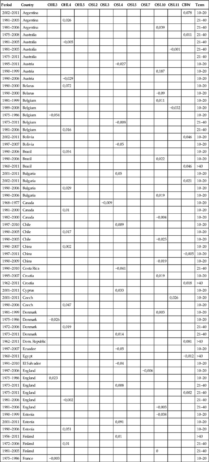

Missende data GDP: Egypt 1959, Croatia 1961–1989, Poland 1961–1984, USA 1945–1959, Finland 1955–1959, Estonia 1989–1994, Czech 1989, Lithuania 1989, Moldavia 1989, Serbia 1995–1996, Belarus 1989.
aSource: Veenhoven and Vergunst, (2014).