1
Getting Started
1.1 How to use this book
Try to put yourself in one of the following categories, then go to the appropriate category heading within this section to find some suggestions about how you might get best value from this book:
- Beginner in both computing and statistics (Section 1.1.1);
- Student needing help with project work (1.1.2);
- Done some R and some statistics, but keen to learn more of both (1.1.3);
- Done regression and ANOVA, but want to learn more advanced statistical modelling (1.1.4);
- Experienced in statistics, but a beginner in R (1.1.5);
- Experienced in computing, but a beginner in R (1.1.6);
- Familiar with statistics and computing, but need a friendly reference manual (1.1.7).
1.1.1 Beginner in both computing and statistics
The book is structured principally with you in mind. There are six key things to learn: how to arrange your data, how to read the data into R, how to check the data once within R, how to select the appropriate statistical model and apply it correctly, how to interpret the output, and how to present the analysis for publication. It is essential that you understand the basics thoroughly before trying to do the more complicated things, so study Chapters 3–6 carefully to begin with. Do all of the exercises that are illustrated in the text on your own computer. Now you need to do the hard part, which is selecting the right statistics to use. Model choice is extremely important, and is the thing that will develop most with experience. Do not by shy to ask for expert help with this. Never do an analysis that is more complicated than it needs to be, so start by reading about the classical tests to see if one of these fits your purposes (Chapter 8). Finally, try to understand the distinction between regression (Chapter 10) where the explanatory variable is continuous, and analysis of variance (Chapter 11), where the explanatory variable is categorical. One of these two is likely to be the most complicated method you will need.
1.1.2 Student needing help with project work
The first thing to ensure is that you know the difference between your response variable and your explanatory variable, and the distinction between a continuous variable and a categorical variable (Chapter 5). Once you have mastered this, then use the key at the beginning of Chapter 9 to see what kind of statistics you need to employ. It is most likely that if your response variable is a count, where you typically have lots of zeros, then you will want to use either the classical tests (Chapter 8) or count data in tables (Chapter 15). If your response variable is a continuous measure (e.g. a weight) then you will want to use either regression (Chapter 10) if your explanatory variable is continuous (e.g. an altitude) or analysis of variance (Chapter 11) if your explanatory variable is categorical (e.g. genotype). Do not forget to use the appropriate graphics (scatter plots for regressions, box and whisker plots for ANOVA).
1.1.3 Done some R and some statistics, but keen to learn more of both
The best plan is to skim quickly through the introductory material in case you have missed out on some of the basics. Certainly you should read all of the material in Chapter 2 on the fundamentals of the R language and Chapter 5 on graphics. Then, if you know what statistical models you want to use, go directly to the relevant chapter (e.g. regression in Chapter 10 and then non-linear regression in Chapter 20). Use the index for finding help on specific topics.
1.1.4 Done regression and ANOVA, but want to learn more advanced statistical modelling
If you learned regression and ANOVA in another language, the best plan is to go directly to Chapters 10–12 to see how the output from linear models is handled by R. Once you have familiarized yourself with data input (Chapter 3) and dataframes (Chapter 4), you should be able to go directly to the chapters on generalized linear models (Chapter 13), spatial statistics (Chapter 26), survival analysis (Chapter 27), non-linear models (Chapter 20) or mixed-effects models (Chapter 19) without any difficulty.
1.1.5 Experienced in statistics, but a beginner in R
The first thing is to get a thorough understanding of dataframes and data input to R, for which you should study Chapters 3 and 4. Then, if you know what statistics you want to do (e.g. mixed-effects models in R), you should be able to go straight to the appropriate material (Chapter 19 in this case). To understand the output from models in R, you will want to browse Chapter 9 on statistical modelling in R. Then you will want to present your data in the most effective way, by reading Chapter 5 on graphics and Chapter 29 on changing the look of graphics.
1.1.6 Experienced in computing, but a beginner in R
Well-written R code is highly intuitive and very readable. The most unfamiliar parts of R are likely to be the way it handles functions and the way it deals with environments. It is impossible to anticipate the order in which more advanced users are likely to encounter material and hence want to learn about specific features of the language, but vectorized calculations, subscripts on dataframes, function-writing and suchlike are bound to crop up early (Chapter 2). If you see a name in some code, and you want to find out about it, just type the name immediately after a question mark at the R prompt >. If, for example, you want know what rnbinom does, type:
?rnbinom
Recognizing mathematical functions is quite straightforward because of their names and the fact that their arguments are enclosed in round brackets (). Subscripts on objects have square brackets [ ]. Multi-line blocks of R code are enclosed within curly brackets { }. Again, you may not be familiar with lists, or with applying functions to lists; elements within lists have double square brackets [[ ]].
Look at the sections at the head of Chapter 2 as a starting point. The index is probably your most sensible entry point for queries about specifics.
1.1.7 Familiar with statistics and computing, but need a friendly reference manual
If it is a topic you want to understand, then use the chapter list on pages v–vi and the Detailed Contents on pp. vii–xxi to find the most appropriate section. For aspects of the R language, look at the sections mentioned at the start of Chapter 2 on p. 12. You are likely to want to spend time browsing the contents of general material such as Chapter 5 on graphics and Chapter 29 on changing the look of graphics. Your best bet, in general, is likely to be to use the Index.
Get used to R's help pages. If you know the name of the function for which you require help, just type a question mark followed directly by the function name at R's screen prompt >. To find out what all the graphics parameters mean, for instance, just type:
?par
1.2 Installing R
I assume that you have a PC or an Apple Mac, and that you want to install R on the hard disc. If you have access to the internet then this could hardly be simpler. First go to the site called CRAN (this stands for Comprehensive R Archive Network). You can type its full address,
http://cran.r-project.org/
or simply type CRAN into Google and be transported effortlessly to the site. Once there, you need to ‘Download and Install R’ by running the appropriate precompiled binary distributions. Click to choose between Linux, Mac OS and Windows, then follow the (slightly different) instructions. You want the ‘base’ package and you want to run the setup program which will have a name like R*.exe (on a PC) or R*.dmg (on a Mac). When asked, say you want to ‘Run’ the file (rather than ‘Save’ it). Then just sit back and watch. If you do not have access to the internet, then get a friend to download R and copy it onto a memory stick for you.
1.3 Running R
To run R, just click on the R icon. If there is no icon, go to Programs, then to R, then click on the R icon. The first thing you see is the version number of R and the date of your version. It is a good idea to visit the CRAN site regularly to make sure that you have got the most up-to-date version of R. If you have an old version, it is best to uninstall your current version before downloading the new one.
The header explains that there is no warranty for this free software, and allows you to see the list of current contributors. Perhaps the most important information in the header is found under
citation()
which shows how to cite the R software in your written work. The R Development Core Team has done a huge amount of work and we, the R user community, should give them due credit whenever we publish work that has used R.
Below the header you will see a blank line with a > symbol in the left-hand margin. This is called the prompt and is R's way of saying ‘What now?’. This is where you type in your commands, as introduced on p. 13. When working, you will sometimes see + at the left-hand side of the screen instead of >. This means that the last command you typed is incomplete. The commonest cause of this is that you have forgotten one or more brackets. If you can see what is missing (e.g. a final right-hand bracket) then just type the missing character and press enter, at which point the command will execute. If you have made a mistake, then press the Esc key and the command line prompt > will reappear. Then use the Up arrow key to retrieve your last command, at which point you can correct the mistake, using the Left and Right arrow keys.
1.4 The Comprehensive R Archive Network
CRAN is your first port of call for everything to do with R. It is from here that you download and install R, find contributed packages to solve particular problems, find the answers to frequently asked questions, read about the latest developments, get programming tips and much more besides. These are the current headings on the main website:
It is well worth browsing through The R Journal (formerly R News). This is the refereed journal of the R project for statistical computing. It features short to medium-length articles covering topics that might be of interest to users or developers of R, including:
- Add-on packages – short introductions to or reviews of R extension packages.
- Programmer's Niche – hints for programming in R.
- Help Desk – hints for newcomers explaining aspects of R that might not be so obvious from reading the manuals and FAQs.
- Applications – demonstrating how a new or existing technique can be applied in an area of current interest using R, providing a fresh view of such analyses in R that is of benefit beyond the specific application.
1.4.1 Manuals
There are several manuals available on CRAN:
- An Introduction to R gives an introduction to the language and how to use R for doing statistical analysis and graphics.
- A draft of the R Language Definition, which documents the language per se – that is, the objects that it works on, and the details of the expression evaluation process, which are useful to know when programming R functions. This is perhaps the most important of all the manuals.
- Writing R Extensions covers how to create your own packages, write R help files, and use the foreign language (C, C++, Fortran, …) interfaces.
- R Data Import/Export describes the import and export facilities available either in R itself or via packages which are available from CRAN.
- R Installation and Administration, which is self-explanatory.
- R: A Language and Environment for Statistical Computing (referred to on the website as ‘The R Reference Index’) contains all the help files of the R standard and recommended packages in printable form.
These manuals are also available in R itself by choosing Help/Manuals (in PDF) from the menu bar. There are also answers to Frequently Asked Questions (FAQs) and The R Journal, as mentioned above. The most useful part of the site, however, is the Search facility which allows you to investigate the contents of most of the R documents, functions, and searchable mail archives.
1.4.2 Frequently asked questions
R has three collections of answers to FAQs:
- the R FAQ, which is the general collection and contains useful information for users on all platforms (Linux, Mac, Unix, Windows);
- the R Mac OS X FAQ for all users of Apple operating systems;
- the R Windows FAQ for all users of Microsoft operating systems.
You need to read the first of these, plus the appropriate one for your platform.
1.4.3 Contributed documentation
This contains a wide range of longer (more than 100 pages) and shorter manuals, tutorials, and exercises provided by users of R. You should browse these to find the ones most relevant to your needs.
1.5 Getting help in R
The simplest way to get help in R is to click on the Help button on the toolbar of the RGui window (this stands for R's Graphic User Interface). Alternatively, if you are connected to the internet, you can type CRAN into Google and search for the help you need at CRAN (see Section 1.4). However, if you know the name of the function you want help with, you just type a question mark ? at the command line prompt followed by the name of the function. So to get help on read.table, just type
?read.table
Sometimes you cannot remember the precise name of the function, but you know the subject on which you want help (e.g. data input in this case). Use the help.search function (without a question mark) with your query in double quotes like this:
help.search("data input")
and (with any luck) you will see the names of the R functions associated with this query. Then you can use ?read.table to get detailed help.
Other useful functions are find and apropos. The find function tells you what package something is in:
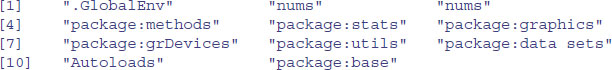
find("lowess")
[1] "package:stats"
while apropos returns a character vector giving the names of all objects in the search list that match your (potentially partial) enquiry:
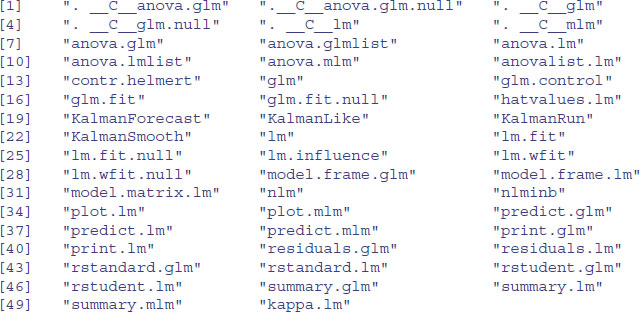
apropos("lm")
1.5.1 Worked examples of functions
To see a worked example just type the function name (e.g. linear models, lm)
example(lm)
and you will see the printed and graphical output produced by the lm function.
1.5.2 Demonstrations of R functions
These can be useful for seeing the range of things that R can do. Here are some for you to try:
demo(persp)
demo(graphics)
demo(Hershey)
demo(plotmath)
1.6 Packages in R
Finding your way around the contributed packages can be tricky, simply because there are so many of them, and the name of the package is not always as indicative of its function as you might hope. There is no comprehensive cross-referenced index, but there is a very helpful feature called ‘Task Views’ on CRAN, which explains the packages available under a limited number of usefully descriptive headings. Click on Packages on the CRAN home page, then inside Contributed Packages, you can click on CRAN Task Views, which allows you to browse bundles of packages assembled by topic. Currently, there are 29 Task Views on CRAN as follows:
| Bayesian | Bayesian Inference |
| ChemPhys | Chemometrics and Computational Physics |
| ClinicalTrials | Clinical Trial Design, Monitoring, and Analysis |
| Cluster | Cluster Analysis & Finite Mixture Models |
| DifferentialEquations | Differential Equations |
| Distributions | Probability Distributions |
| Econometrics | Computational Econometrics |
| Environmetrics | Analysis of Ecological and Environmental Data |
| ExperimentalDesign | Design of Experiments (DoE) & Analysis of Experimental Data |
| Finance | Empirical Finance |
| Genetics | Statistical Genetics |
| Graphics | Graphic Displays & Dynamic Graphics & Graphic Devices & Visualization |
| HighPerformanceComputing | High-Performance and Parallel Computing with R |
| MachineLearning | Machine Learning & Statistical Learning |
| MedicalImaging | Medical Image Analysis |
| Multivariate | Multivariate Statistics |
| NaturalLanguageProcessing | Natural Language Processing |
| OfficialStatistics | Official Statistics & Survey Methodology |
| Optimization | Optimization and Mathematical Programming |
| Pharmacokinetics | Analysis of Pharmacokinetic Data |
| Phylogenetics | Phylogenetics, Especially Comparative Methods |
| Psychometrics | Psychometric Models and Methods |
| ReproducibleResearch | Reproducible Research |
| Robust | Robust Statistical Methods |
| SocialSciences | Statistics for the Social Sciences |
| Spatial | Analysis of Spatial Data |
| Survival | Survival Analysis |
| TimeSeries | Time Series Analysis |
| gR | gRaphical Models in R |
Click on the Task View to get an annotated list of the packages available under any particular heading. With any luck you will find the package you are looking for.
To use one of the built-in libraries (listed in Table 1.1 ), simply type the library function with the name of the library in brackets. Thus, to load the spatial library type:
Table 1.1 Libraries used in this book that come supplied as part of the base package of R.
| lattice | lattice graphics for panel plots or trellis graphs |
| MASS | package associated with Venables and Ripley's book entitled Modern Applied Statistics using S-PLUS |
| mgcv | generalized additive models |
| nlme | mixed-effects models (both linear and non-linear) |
| nnet | feed-forward neural networks and multinomial log-linear models |
| spatial | functions for kriging and point pattern analysis |
| survival | survival analysis, including penalised likelihood |
library(spatial)
1.6.1 Contents of packages
It is easy to use the help function to discover the contents of library packages. Here is how you find out about the contents of the spatial library:
library(help=spatial)
| Information on package "spatial" | |
| Package: | spatial |
| Description: | Functions for kriging and point pattern analysis. |
followed by a list of all the functions and data sets. You can view the full list of the contents of a library using objects with search() like this. Here are the contents of the spatial library:
objects(grep("spatial",search()))
Then, to find out how to use, say, Ripley's K (Kfn), just type:
?Kfn
1.6.2 Installing packages
The base package does not contain some of the libraries referred to in this book, but downloading these is very simple. Before you start, you should check whether you need to “Run as administrator” before you can install packages (right click on the R icon to find this). Run the R program, then from the command line use the install.packages function to download the libraries you want. You will be asked to highlight the mirror nearest to you for fast downloading (e.g. London), then everything else is automatic. The packages used in this book are
install.packages("akima")
install.packages("boot")
install.packages("car")
install.packages("lme4")
install.packages("meta")
install.packages("mgcv")
install.packages("nlme")
install.packages("deSolve")
install.packages("R2jags")
install.packages("RColorBrewer")
install.packages("RODBC")
install.packages("rpart")
install.packages("spatstat")
install.packages("spdep")
install.packages("tree")
If you want other packages, then go to CRAN and browse the list called ‘Packages’ to select the ones you want to investigate.
1.7 Command line versus scripts
When writing functions and other multi-line sections of input you will find it useful to use a text editor rather than execute everything directly at the command line. Some people prefer to use R's own built-in editor. It is accessible from the RGui menu bar. Click on File then click on New script. At this point R will open a window entitled Untitled - R Editor. You can type and edit in this, then when you want to execute a line or group of lines, just highlight them and press Ctrl+R (the Control key and R together). The lines are automatically transferred to the command window and executed.
By pressing Ctrl+S you can save the contents of the R Editor window in a file that you will have to name. It will be given a .R file extension automatically. In a subsequent session you can click on File/Open script…when you will see all your saved .R files and can select the one you want to open.
Other people prefer to use an editor with more features. Tinn-R (“this is not notepad” for R) is very good, or you might like to try RStudio, which has the nice feature of allowing you to scroll back through all of the graphics produced in a session. These and others are free to download from the web.
1.8 Data editor
There is a data editor within R that can be accessed from the menu bar by selecting Edit/Data editor…. You provide the name of the matrix or dataframe containing the material you want to edit (this has to be a dataframe that is active in the current R session, rather than one which is stored on file), and a Data Editor window appears. Alternatively, you can do this from the command line using the fix function (e.g. fix(data.frame.name)). Suppose you want to edit the bacteria dataframe which is part of the MASS library:
library(MASS)
attach(bacteria)
fix(bacteria)
The window has the look of a spreadsheet, and you can change the contents of the cells, navigating with the cursor or with the arrow keys. My preference is to do all of my data preparation and data editing in a spreadsheet before even thinking about using R. Once checked and edited, I save the data from the spreadsheet to a tab-delimited text file (*.txt) that can be imported to R very simply using the function called read.table (p. 20). One of the most persistent frustrations for beginners is that they cannot get their data imported into R. Things that typically go wrong at the data input stage and the necessary remedial actions are described on p. 139.
1.9 Changing the look of the R screen
The default settings of the command window are inoffensive to most people, but you can change them if you do not like them. The Rgui Configuration Editor under Edit/GUI preferences…is used to change the look of the screen. You can change the colour of the input line (default is red), the output line (default navy) or the background (default white). The default numbers of rows (25) and columns (80) can be changed, and you have control over the font (default Courier New) and font size (default 10).
1.10 Good housekeeping
To see what variables you have created in the current session, type:
objects()

To see which packages and dataframes are currently attached:
search()
At the end of a session in R, it is good practice to remove (rm) any variables names you have created (using, say, x <- 5.6) and to detach any dataframes you have attached earlier in the session. That way, variables with the same names but different properties will not get in each other's way in subsequent work:
rm(x,y,z)
detach(worms)
The detach command does not make the dataframe called worms disappear; it just means that the variables within worms, such as Slope and Area, are no longer accessible directly by name. To get rid of everything, including all the dataframes, type
rm(list=ls())
but be absolutely sure that you really want to be as draconian as this before you execute the command.
1.11 Linking to other computer languages
Advanced users can employ the functions .C and .Fortran to provide a standard interface to compiled code that has been linked into R, either at build time or via dyn.load. They are primarily intended for compiled C and Fortran code respectively, but the .C function can be used with other languages which can generate C interfaces, for example C++. The .Internal and .Primitive interfaces are used to call C code compiled into R at build time. Functions .Call and .External provide interfaces which allow compiled code (primarily compiled C code) to manipulate R objects.