2
Essentials of the R Language
There is an enormous range of things that R can do, and one of the hardest parts of learning R is finding your way around. Likewise, there is no obvious order in which different people will want to learn the different components of the R language. I suggest that you quickly scan down the following bullet points, which represent the order in which I have chosen to present the introductory material, and if you are relatively experienced in statistical computing, you might want to skip directly to the relevant section. I strongly recommend that beginners work thorough the material in the order presented, because successive sections build upon knowledge gained from previous sections. This chapter is divided into the following sections:
- 2.1 Calculations
- 2.2 Logical operations
- 2.3 Sequences
- 2.4 Testing and coercion
- 2.5 Missing values and things that are not numbers
- 2.6 Vectors and subscripts
- 2.7 Vectorized functions
- 2.8 Matrices and arrays
- 2.9 Sampling
- 2.10 Loops and repeats
- 2.11 Lists
- 2.12 Text, character strings and pattern matching
- 2.13 Dates and times
- 2.14 Environments
- 2.15 Writing R functions
- 2.16 Writing to file from R
Other essential material is elsewhere: beginners will want to master data input (Chapter 3), dataframes (Chapter 4) and graphics (Chapter 5).
2.1 Calculations
The screen prompt > is an invitation to put R to work. The convention in this book is that material that you need to type into the command line after the screen prompt is shown in red in Courier New font. Just press the Return key to see the answer. You can use the command line as a calculator, like this:
> log(42/7.3)
[1] 1.749795
Each line can have at most 8192 characters, but if you want to see a lengthy instruction or a complicated expression on the screen, you can continue it on one or more further lines simply by ending the line at a place where the line is obviously incomplete (e.g. with a trailing comma, operator, or with more left parentheses than right parentheses, implying that more right parentheses will follow). When continuation is expected, the prompt changes from > to +, as follows:
> 5+6+3+6+4+2+4+8+
+ 3+2+7
[1] 50
Note that the + continuation prompt does not carry out arithmetic plus. If you have made a mistake, and you want to get rid of the + prompt and return to the > prompt, then press the Esc key and use the Up arrow to edit the last (incomplete) line.
From here onwards and throughout the book, the prompt character > will be omitted. The output from R is shown in blue in Courier New font, which uses absolute rather than proportional spacing, so that columns of numbers remain neatly aligned on the page or on the screen.
Two or more expressions can be placed on a single line so long as they are separated by semi-colons:
2+3; 5*7; 3-7
[1] 5
[1] 35
[1] -4
For very big numbers or very small numbers R uses the following scheme (called exponents):
| 1.2e3 | means 1200 because the e3 means ‘move the decimal point 3 places to the right’; |
| 1.2e-2 | means 0.012 because the e-2 means ‘move the decimal point 2 places to the left’; |
| 3.9+4.5i | is a complex number with real (3.9) and imaginary (4.5) parts, and i is the square root of –1. |
2.1.1 Complex numbers in R
Complex numbers consist of a real part and an imaginary part, which is identified by lower-case i like this:
z <- 3.5-8i
The elementary trigonometric, logarithmic, exponential, square root and hyperbolic functions are all implemented for complex values. The following are the special R functions that you can use with complex numbers. Determine the real part:
Re(z)
[1] 3.5
Determine the imaginary part:
Im(z)
[1] -8
Calculate the modulus (the distance from z to 0 in the complex plane by Pythagoras; if x is the real part and y is the imaginary part, then the modulus is  ):
):
Mod(z)
[1] 8.732125
Calculate the argument (Arg(x+ yi)= atan(y/x)):
Arg(z)
[1] -1.158386
Work out the complex conjugate (change the sign of the imaginary part):
Conj(z)
[1] 3.5+8i
Membership and coercion are dealt with in the usual way (p. 30):
is.complex(z)
[1] TRUE
as.complex(3.8)
[1] 3.8+0i
2.1.2 Rounding
Various sorts of rounding (rounding up, rounding down, rounding to the nearest integer) can be done easily. Take the number 5.7 as an example. The ‘greatest integer less than’ function is floor:
floor(5.7)
[1] 5
The ‘next integer’ function is ceiling:
ceiling(5.7)
[1] 6
You can round to the nearest integer by adding 0.5 to the number, then using floor. There is a built-in function for this, but we can easily write one of our own to introduce the notion of function writing. Call it rounded, then define it as a function like this:
rounded <- function(x) floor(x+0.5)
Now we can use the new function:
rounded(5.7)
[1] 6
rounded(5.4)
[1] 5
The hard part is deciding how you want to round negative numbers, because the concept of up and down is more subtle (remember that –5 is a bigger number than –6). You need to think, instead, of whether you want to round towards zero or away from zero. For negative numbers, rounding up means rounding towards zero so do not be surprised when the value of the positive part is different:
ceiling(-5.7)
[1] -5
With floor, negative values are rounded away from zero:
floor(-5.7)
[1] -6
You can simply strip off the decimal part of the number using the function trunc, which returns the integers formed by truncating the values in x towards zero:
trunc(5.7)
[1] 5
trunc(-5.7)
[1] -5
There is an R function called round that you can use by specifying 0 decimal places in the second argument:
round(5.7,0)
[1] 6
round(5.5,0)
[1] 6
round(5.4,0)
[1] 5
round(-5.7,0)
[1] -6
The number of decimal places is not the same as the number of significant digits. You can control the number of significant digits in a number using the function signif. Take a big number like 12 345 678 (roughly 12.35 million). Here is what happens when we ask for 4, 5 or 6 significant digits:
signif(12345678,4)
[1] 12350000
signif(12345678,5)
[1] 12346000
signif(12345678,6)
[1] 12345700
and so on. Why you would want to do this would need to be explained.
2.1.3 Arithmetic
The screen prompt in R is a fully functional calculator. You can add and subtract using the obvious + and - symbols, while division is achieved with a forward slash / and multiplication is done by using an asterisk * like this:
7 + 3 - 5 * 2
[1] 0
Notice from this example that multiplication (5 × 2) is done before the additions and subtractions. Powers (like squared or cube root) use the caret symbol ^ and are done before multiplication or division, as you can see from this example:
3^2 / 2
[1] 4.5
All the mathematical functions you could ever want are here (see Table 2.1). The log function gives logs to the base e (e = 2.718 282), for which the antilog function is exp:
Table 2.1 Mathematical functions used in R.
| Function | Meaning |
| log(x) | log to base e of x |
| exp(x) | antilog of x (ex) |
| log(x,n) | log to base n of x |
| log10(x) | log to base 10 of x |
| sqrt(x) | square root of x |
| factorial(x) | 
|
| choose(n,x) | binomial coefficients n!/(x! (n – x)!) |
| gamma(x) | Γ(x), for real x (x–1)!, for integer x |
| lgamma(x) | natural log of Γ(x) |
| floor(x) | greatest integer less than x |
| ceiling(x) | smallest integer greater than x |
| trunc(x) | closest integer to x between x and 0, e.g. trunc(1.5) = 1, trunc(–1.5) = –1; trunc is like floor for positive values and like ceiling for negative values |
| round(x, digits=0) | round the value of x to an integer |
| signif(x, digits=6) | give x to 6 digits in scientific notation |
| runif(n) | generates n random numbers between 0 and 1 from a uniform distribution |
| cos(x) | cosine of x in radians |
| sin(x) | sine of x in radians |
| tan(x) | tangent of x in radians |
| acos(x), asin(x), atan(x) | inverse trigonometric transformations of real or complex numbers |
| acosh(x), asinh(x), atanh(x) | inverse hyperbolic trigonometric transformations of real or complex numbers |
| abs(x) | the absolute value of x, ignoring the minus sign if there is one |
log(10)
[1] 2.302585
exp(1)
[1] 2.718282
If you are old fashioned, and want logs to the base 10, then there is a separate function, log10:
log10(6)
[1] 0.7781513
Logs to other bases are possible by providing the log function with a second argument which is the base of the logs you want to take. Suppose you want log to base 3 of 9:
log(9,3)
[1] 2
The trigonometric functions in R measure angles in radians. A circle is 2π radians, and this is 360°, so a right angle (90°) is π/2 radians. R knows the value of π as pi:
pi
[1] 3.141593
sin(pi/2)
[1] 1
cos(pi/2)
[1] 6.123032e-017
Notice that the cosine of a right angle does not come out as exactly zero, even though the sine came out as exactly 1. The e-017 means ‘times 10–17’. While this is a very small number, it is clearly not exactly zero (so you need to be careful when testing for exact equality of real numbers; see p. 23).
2.1.4 Modulo and integer quotients
Integer quotients and remainders are obtained using the notation %/% (percent, divide, percent) and %% (percent, percent) respectively. Suppose we want to know the integer part of a division: say, how many 13s are there in 119:
119 %/% 13
[1] 9
Now suppose we wanted to know the remainder (what is left over when 119 is divided by 13): in maths this is known as modulo:
119 %% 13
[1] 2
Modulo is very useful for testing whether numbers are odd or even: odd numbers have modulo 2 value 1 and even numbers have modulo 2 value 0:
9 %% 2
[1] 1
8 %% 2
[1] 0
Likewise, you use modulo to test if one number is an exact multiple of some other number. For instance, to find out whether 15 421 is a multiple of 7 (which it is), then ask:
15421 %% 7 == 0
[1] TRUE
Note the use of ‘double equals’ to test for equality (this is explained in detail on p. 26).
2.1.5 Variable names and assignment
There are three important things to remember when selecting names for your variables in R:
- Variable names in R are case sensitive, so y is not the same as Y.
- Variable names should not begin with numbers (e.g. 1x) or symbols (e.g. %x).
- Variable names should not contain blank spaces (use back.pay not back pay).
In terms of your work–life balance, make your variable names as short as possible, so that you do not spend most of your time typing, and the rest of your time correcting spelling mistakes in your ridiculously long variable names.
Objects obtain values in R by assignment (‘x gets a value’). This is achieved by the gets arrow <- which is a composite symbol made up from ‘less than’ and ‘minus’ with no space between them. Thus, to create a scalar constant x with value 5 we type:
x <- 5
and not x = 5. Notice that there is a potential ambiguity if you get the spacing wrong. Compare our x <- 5, ‘x gets 5’, with x < - 5 where there is a space between the ‘less than’ and ‘minus’ symbol. In R, this is actually a question, asking ‘is x less than minus 5?’ and, depending on the current value of x, would evaluate to the answer either TRUE or FALSE.
2.1.6 Operators
R uses the following operator tokens:
| + - * / %/% %% ^ | arithmetic (plus, minus, times, divide, integer quotient, modulo, power) |
| >= < <= == != | relational (greater than, greater than or equals, less than, less than or equals, equals, not equals) |
| ! & | | logical (not, and, or) |
| ~ | model formulae (‘is modelled as a function of’) |
| <- -> | assignment (gets) |
| $ | list indexing (the ‘element name’ operator) |
| : | create a sequence |
Several of these operators have different meaning inside model formulae. Thus * indicates the main effects plus interaction (rather than multiplication), : indicates the interaction between two variables (rather than generate a sequence) and ^ means all interactions up to the indicated power (rather than raise to the power). You will learn more about these ideas in Chapter 9.
2.1.7 Integers
Integer vectors exist so that data can be passed to C or Fortran code which expects them, and so that small integer data can be represented exactly and compactly. The range of integers is from −2 000 000 000 to +2 000 000 000 (-2*10^9 to +2*10^9, which R could portray as -2e+09 to 2e+09).
Be careful. Do not try to change the class of a vector by using the integer function. Here is a numeric vector of whole numbers that you want to convert into a vector of integers:
x <- c(5,3,7,8)
is.integer(x)
[1] FALSE
is.numeric(x)
[1] TRUE
Applying the integer function to it replaces all your numbers with zeros; definitely not what you intended.
x <- integer(x)
x
[1] 0 0 0 0 0
Make the numeric object first, then convert the object to integer using the as.integer function like this:
x <- c(5,3,7,8)
x <- as.integer(x)
is.integer(x)
[1] TRUE
The integer function works as trunc when applied to real numbers, and removes the imaginary part when applied to complex numbers:
as.integer(5.7)
[1] 5
as.integer(-5.7)
[1] -5
as.integer(5.7 -3i)
[1] 5
Warning message:
imaginary parts discarded in coercion
2.1.8 Factors
Factors are categorical variables that have a fixed number of levels. A simple example of a factor might be a variable called gender with two levels: ‘female’ and ‘male’. If you had three females and two males, you could create the factor like this:
gender <- factor(c("female", "male", "female", "male", "female"))
class(gender)
[1] "factor"
mode(gender)
[1] "numeric"
More often, you will create a dataframe by reading your data from a file using read.table. When you do this, all variables containing one or more character strings will be converted automatically into factors. Here is an example:
data <- read.table("c:\\temp\\daphnia.txt",header=T)
attach(data)
head(data)
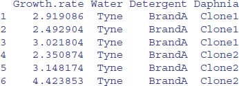
This dataframe contains a continuous response variable (Growth.rate) and three categorical explanatory variables (Water, Detergent and Daphnia), all of which are factors. In statistical modelling, factors are associated with analysis of variance (all the explanatory variables are categorical) and analysis of covariance (some of the explanatory variables are categorical and some are continuous).
There are some important functions for dealing with factors. You will often want to check that a variable is a factor (especially if the factor levels are numbers rather than characters):
is.factor(Water)
[1] TRUE
To discover the names of the factor levels, we use the levels function:
levels(Detergent)
[1] "BrandA" "BrandB" "BrandC" "BrandD"
To discover the number of levels of a factor, we use the nlevels function:
nlevels(Detergent)
[1] 4
The same result is achieved by applying the length function to the levels of a factor:
length(levels(Detergent))
[1] 4
By default, factor levels are treated in alphabetical order. If you want to change this (as you might, for instance, in ordering the bars of a bar chart) then this is straightforward: just type the factor levels in the order that you want them to be used, and provide this vector as the second argument to the factor function.
Suppose we have an experiment with three factor levels in a variable called treatment, and we want them to appear in this order: ‘nothing’, ‘single’ dose and ‘double’ dose. We shall need to override R's natural tendency to order them ‘double’, ‘nothing’, ‘single’:
frame <- read.table("c:\\temp\\trial.txt",header=T)
attach(frame)
tapply(response,treatment,mean)
double nothing single
25 60 34
This is achieved using the factor function like this:
treatment <- factor(treatment,levels=c("nothing","single","double"))
Now we get the order we want:
tapply(response,treatment,mean)
nothing single double
60 34 25
Only == and != can be used for factors. Note, also, that a factor can only be compared to another factor with an identical set of levels (not necessarily in the same ordering) or to a character vector. For example, you cannot ask quantitative questions about factor levels, like > or <=, even if these levels are numeric.
To turn factor levels into numbers (integers) use the unclass function like this:
as.vector(unclass(Daphnia))
[1] 1 1 1 2 2 2 3 3 3 1 1 1 2 2 2 3 3 3 1 1 1 2 2 2 3 3 3 1 1 1 2 2 2 3 3 3 1 1
[39] 1 2 2 2 3 3 3 1 1 1 2 2 2 3 3 3 1 1 1 2 2 2 3 3 3 1 1 1 2 2 2 3 3 3
2.2 Logical operations
A crucial part of computing involves asking questions about things. Is one thing bigger than other? Are two things the same size? Questions can be joined together using words like ‘and’ ‘or’, ‘not’. Questions in R typically evaluate to TRUE or FALSE but there is the option of a ‘maybe’ (when the answer is not available, NA). In R, < means ‘less than’, > means ‘greater than’, and ! means ‘not’ (see Table 2.2).
Table 2.2 Logical and relational operations.
| Symbol | Meaning |
| ! | logical NOT |
| & | logical AND |
| | | logical OR |
| < | less than |
| <= | less than or equal to |
| > | greater than |
| = | greater than or equal to |
| == | logical equals (double =) |
| != | not equal |
| && | AND with IF |
| || | OR with IF |
| xor(x,y) | exclusive OR |
| isTRUE(x) | an abbreviation of identical(TRUE,x) |
2.2.1 TRUE and T with FALSE and F
You can use T for TRUE and F for FALSE, but you should be aware that T and F might have been allocated as variables. So this is obvious:
TRUE == FALSE
[1] FALSE
T == F
[1] FALSE
This, however, is not so obvious:
T <- 0
T == FALSE
[1] TRUE
F <- 1
TRUE == F
[1] TRUE
But now, of course, T is not equal to F:
T != F
[1] TRUE
To be sure, always write TRUE and FALSE in full, and never use T or F as variable names.
2.2.2 Testing for equality with real numbers
There are international standards for carrying out floating point arithmetic, but on your computer these standards are beyond the control of R. Roughly speaking, integer arithmetic will be exact between –1016 and 1016, but for fractions and other real numbers we lose accuracy because of round-off error. This is only likely to become a real problem in practice if you have to subtract similarly sized but very large numbers. A dramatic loss in accuracy under these circumstances is called ‘catastrophic cancellation error’. It occurs when an operation on two numbers increases relative error substantially more than it increases absolute error.
You need to be careful in programming when you want to test whether or not two computed numbers are equal. R will assume that you mean ‘exactly equal’, and what that means depends upon machine precision. Most numbers are rounded to an accuracy of 53 binary digits. Typically therefore, two floating point numbers will not reliably be equal unless they were computed by the same algorithm, and not always even then. You can see this by squaring the square root of 2: surely these values are the same?
x <- sqrt(2)
x * x == 2
[1] FALSE
In fact, they are not the same. We can see by how much the two values differ by subtraction:
x * x - 2
[1] 4.440892e-16
This is not a big number, but it is not zero either. So how do we test for equality of real numbers? The best advice is not to do it. Try instead to use the alternatives ‘less than’ with ‘greater than or equal to’, or conversely ‘greater than’ with ‘less than or equal to’. Then you will not go wrong. Sometimes, however, you really do want to test for equality. In those circumstances, do not use double equals to test for equality, but employ the all.equal function instead.
2.2.3 Equality of floating point numbers using all.equal
The nature of floating point numbers used in computing is the cause of some initially perplexing features. You would imagine that since 0.3 minus 0.2 is 0.1, and the logic presented below would evaluate to TRUE. Not so:
x <- 0.3 - 0.2
y <- 0.1
x == y
[1] FALSE
The function called identical gives the same result.
identical(x,y)
[1] FALSE
The solution is to use the function called all.equal which allows for insignificant differences:
all.equal(x,y)
[1] TRUE
Do not use all.equal directly in if expressions. Either use isTRUE(all.equal(….)) or identical as appropriate.
2.2.4 Summarizing differences between objects using all.equal
The function all.equal is very useful in programming for checking that objects are as you expect them to be. Where differences occur, all.equal does a useful job in describing all the differences it finds. Here, for instance, it reports on the difference between a which is a vector of characters and b which is a factor:
a <- c("cat","dog","goldfish")
b <- factor(a)
In the all.equal function, the object on the left (a) is called the ‘target’ and the object on the right (b) is ‘current’:
all.equal(a,b)
[1] "Modes: character, numeric"
[2] "Attributes: < target is NULL, current is list >"
[3] "target is character, current is factor"
Recall that factors are stored internally as integers, so they have mode = numeric.
class(b)
[1] "factor"
mode(b)
[1] "numeric"
The reason why ‘current is list’ in line [2] of the output is that factors have two attributes and these are stored as a list – namely, their levels and their class:
attributes(b)
$levels
[1] "cat" "dog" "goldfish"
$class
[1] "factor"
The all.equal function is also useful for obtaining feedback on differences in things like the lengths of vectors:
n1 <- c(1,2,3)
n2 <- c(1,2,3,4)
all.equal(n1,n2)
[1] "Numeric: lengths (3, 4) differ"
It works well, too, for multiple differences:
n2 <- as.character(n2)
all.equal(n1,n2)
[1] "Modes: numeric, character"
[2] "Lengths: 3, 4"
[3] "target is numeric, current is character"
Note that ‘target’ is the first argument to the function and ‘current’ is the second. If you supply more than two objects to be compared, the third and subsequent objects are simply ignored.
2.2.5 Evaluation of combinations of TRUE and FALSE
It is important to understand how combinations of logical variables evaluate, and to appreciate how logical operations (such as those in Table 2.2) work when there are missing values, NA. Here are all the possible outcomes expressed as a logical vector called x:
x <- c(NA, FALSE, TRUE)
names(x) <- as.character(x)
To see the logical combinations of & (logical AND) we can use the outer function with x to evaluate all nine combinations of NA, FALSE and TRUE like this:
outer(x, x, "&")
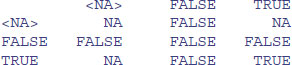
Only TRUE & TRUE evaluates to TRUE. Note the behaviour of NA & NA and NA & TRUE. Where one of the two components is NA, the result will be NA if the outcome is ambiguous. Thus, NA & TRUE evaluates to NA, but NA & FALSE evaluates to FALSE. To see the logical combinations of | (logical OR) write:
outer(x, x, "|")
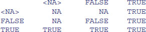
Only FALSE | FALSE evaluates to FALSE. Note the behaviour of NA | NA and NA | FALSE.
2.2.6 Logical arithmetic
Arithmetic involving logical expressions is very useful in programming and in selection of variables. If logical arithmetic is unfamiliar to you, then persevere with it, because it will become clear how useful it is, once the penny has dropped. The key thing to understand is that logical expressions evaluate to either true or false (represented in R by TRUE or FALSE), and that R can coerce TRUE or FALSE into numerical values: 1 for TRUE and 0 for FALSE. Suppose that x is a sequence from 0 to 6 like this:
x <- 0:6
Now we can ask questions about the contents of the vector called x. Is x less than 4?
x < 4
[1] TRUE TRUE TRUE TRUE FALSE FALSE FALSE
The answer is yes for the first four values (0, 1, 2 and 3) and no for the last three (4, 5 and 6). Two important logical functions are all and any. They check an entire vector but return a single logical value: TRUE or FALSE. Are all the x values bigger than 0?
all(x>0)
[1] FALSE
No. The first x value is a zero. Are any of the x values negative?
any(x<0)
[1] FALSE
No. The smallest x value is a zero.
We can use the answers of logical functions in arithmetic. We can count the true values of (x<4), using sum:
sum(x<4)
[1] 4
We can multiply (x<4) by other vectors:
(x<4)*runif(7)
[1] 0.9433433 0.9382651 0.6248691 0.9786844 0.0000000 0.0000000
[7] 0.0000000
Logical arithmetic is particularly useful in generating simplified factor levels during statistical modelling. Suppose we want to reduce a five-level factor (a, b, c, d, e) called treatment to a three-level factor called t2 by lumping together the levels a and e (new factor level 1) and c and d (new factor level 3) while leaving b distinct (with new factor level 2):
(treatment <- letters[1:5])
[1] "a" "b" "c" "d" "e"
(t2 <- factor(1+(treatment=="b")+2*(treatment=="c")+2*(treatment=="d")))
[1] 1 2 3 3 1
Levels: 1 2 3
The new factor t2 gets a value 1 as default for all the factors levels, and we want to leave this as it is for levels a and e. Thus, we do not add anything to the 1 if the old factor level is a or e. For old factor level b, however, we want the result that t2=2 so we add 1 (treatment=="b") to the original 1 to get the answer we require. This works because the logical expression evaluates to 1 (TRUE) for every case in which the old factor level is b and to 0 (FALSE) in all other cases. For old factor levels c and d we want the result that t2=3 so we add 2 to the baseline value of 1 if the original factor level is either c (2*(treatment=="c")) or d (2*(treatment=="d")). You may need to read this several times before the penny drops. Note that ‘logical equals’ is a double equals sign without a space in between (==). You need to understand the distinction between:
| x <- y | x is assigned the value of y (x gets the values of y); |
| x = y | in a function or a list x is set to y unless you specify otherwise; |
| x == y | produces TRUE if x is exactly equal to y and FALSE otherwise. |
2.3 Generating sequences
An important way of creating vectors is to generate a sequence of numbers. The simplest sequences are in steps of 1, and the colon operator is the simplest way of generating such sequences. All you do is specify the first and last values separated by a colon. Here is a sequence from 0 up to 10:
0:10
[1] 0 1 2 3 4 5 6 7 8 9 10
Here is a sequence from 15 down to 5:
15:5
[1] 15 14 13 12 11 10 9 8 7 6 5
To generate a sequence in steps other than 1, you use the seq function. There are various forms of this, of which the simplest has three arguments: from, to, by (the initial value, the final value and the increment). If the initial value is smaller than the final value, the increment should be positive, like this:
seq(0, 1.5, 0.1)
[1] 0.0 0.1 0.2 0.3 0.4 0.5 0.6 0.7 0.8 0.9 1.0 1.1 1.2 1.3 1.4 1.5
If the initial value is larger than the final value, the increment should be negative, like this:
seq(6,4,-0.2)
[1] 6.0 5.8 5.6 5.4 5.2 5.0 4.8 4.6 4.4 4.2 4.0
In many cases, you want to generate a sequence to match an existing vector in length. Rather than having to figure out the increment that will get from the initial to the final value and produce a vector of exactly the appropriate length, R provides the along and length options. Suppose you have a vector of population sizes:
N <- c(55,76,92,103,84,88,121,91,65,77,99)
You need to plot this against a sequence that starts at 0.04 in steps of 0.01:
seq(from=0.04,by=0.01,length=11)
[1] 0.04 0.05 0.06 0.07 0.08 0.09 0.10 0.11 0.12 0.13 0.14
But this requires you to figure out the length of N. A simpler method is to use the along argument and specify the vector, N, whose length has to be matched:
seq(0.04,by=0.01,along=N)
[1] 0.04 0.05 0.06 0.07 0.08 0.09 0.10 0.11 0.12 0.13 0.14
Alternatively, you can get R to work out the increment (0.01 in this example), by specifying the start and the end values (from and to), and the name of the vector (N) whose length has to be matched:
seq(from=0.04,to=0.14,along=N)
[1] 0.04 0.05 0.06 0.07 0.08 0.09 0.10 0.11 0.12 0.13 0.14
An important application of the last option is to get the x values for drawing smooth lines through a scatterplot of data using predicted values from a model (see p. 207).
Notice that when the increment does not match the final value, then the generated sequence stops short of the last value (rather than overstepping it):
seq(1.4,2.1,0.3)
[1] 1.4 1.7 2.0
If you want a vector made up of sequences of unequal lengths, then use the sequence function. Suppose that most of the five sequences you want to string together are from 1 to 4, but the second one is 1 to 3 and the last one is 1 to 5, then:
sequence(c(4,3,4,4,4,5))
[1] 1 2 3 4 1 2 3 1 2 3 4 1 2 3 4 1 2 3 4 1 2 3 4 5
2.3.1 Generating repeats
You will often want to generate repeats of numbers or characters, for which the function is rep. The object that is named in the first argument is repeated a number of times as specified in the second argument. At its simplest, we would generate five 9s like this:
rep(9,5)
[1] 9 9 9 9 9
You can see the issues involved by a comparison of these three increasingly complicated uses of the rep function:
rep(1:4, 2)
[1] 1 2 3 4 1 2 3 4
rep(1:4, each = 2)
[1] 1 1 2 2 3 3 4 4
rep(1:4, each = 2, times = 3)
[1] 1 1 2 2 3 3 4 4 1 1 2 2
[13] 3 3 4 4 1 1 2 2 3 3 4 4
In the simplest case, the entire first argument is repeated (i.e. the sequence 1 to 4 appears twice). You often want each element of the sequence to be repeated, and this is accomplished with the each argument. Finally, you might want each number repeated and the whole series repeated a certain number of times (here three times).
When each element of the series is to be repeated a different number of times, then the second argument must be a vector of the same length as the vector comprising the first argument (length 4 in this example). So if we want one 1, two 2s, three 3s and four 4s we would write:
rep(1:4,1:4)
[1] 1 2 2 3 3 3 4 4 4 4
In a more complicated case, there is a different but irregular repeat of each of the elements of the first argument. Suppose that we need four 1s, one 2, four 3s and two 4s. Then we use the concatenation function c to create a vector of length 4 c(4,1,4,2) which will act as the second argument to the rep function:
rep(1:4,c(4,1,4,2))
[1] 1 1 1 1 2 3 3 3 3 4 4
Here is the most complex case with character data rather than numbers: each element of the series is repeated an irregular number of times:
rep(c("cat","dog","gerbil","goldfish","rat"),c(2,3,2,1,3))
[1] "cat" "cat" "dog" "dog" "dog" "gerbil"
[7] "gerbil" "goldfish" "rat" "rat" "rat"
This is the most general, and also the most useful form of the rep function.
2.3.2 Generating factor levels
The function gl (‘generate levels’) is useful when you want to encode long vectors of factor levels. The syntax for the three arguments is: ‘up to’, ‘with repeats of’, ‘to total length’. Here is the simplest case where we want factor levels up to 4 with repeats of 3 repeated only once (i.e. to total length 12):
gl(4,3)
[1] 1 1 1 2 2 2 3 3 3 4 4 4
Levels: 1 2 3 4
Here is the function when we want that whole pattern repeated twice:
gl(4,3,24)
[1] 1 1 1 2 2 2 3 3 3 4 4 4
[13] 1 1 1 2 2 2 3 3 3 4 4 4
Levels: 1 2 3 4
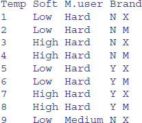
If you want text for the factor levels, rather than numbers, use labels like this:
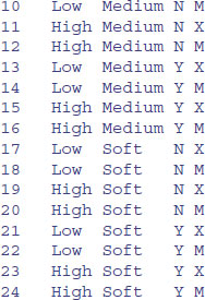
Temp <- gl(2, 2, 24, labels = c("Low", "High"))
Soft <- gl(3, 8, 24, labels = c("Hard","Medium","Soft"))
M.user <- gl(2, 4, 24, labels = c("N", "Y"))
Brand <- gl(2, 1, 24, labels = c("X", "M"))
data.frame(Temp,Soft,M.user,Brand)
2.4 Membership: Testing and coercing in R
The concepts of membership and coercion may be unfamiliar. Membership relates to the class of an object in R. Coercion changes the class of an object. For instance, a logical variable has class logical and mode logical. This is how we create the variable:
lv <- c(T,F,T)
We can assess its membership by asking if it is a logical variable using the is.logical function:
is.logical(lv)
[1] TRUE
It is not a factor, and so it does not have levels:
levels(lv)
NULL
But we can coerce it be a two-level factor like this:
(fv <- as.factor(lv))
[1] TRUE FALSE TRUE
Levels: FALSE TRUE
is.factor(fv)
[1] TRUE
We can coerce a logical variable to be numeric: TRUE evaluates to 1 and FALSE evaluates to zero, like this:
(nv <- as.numeric(lv))
[1] 1 0 1
This is particularly useful as a shortcut when creating new factors with reduced numbers of levels (as we do in model simplification).
In general, the expression as(object, value) is the way to coerce an object to a particular class. Membership functions ask is.something and coercion functions say as.something.
Objects have a type, and you can test the type of an object using an is.type function (Table 2.3). For instance, mathematical functions expect numeric input and text-processing functions expect character input. Some types of objects can be coerced into other types. A familiar type of coercion occurs when we interpret the TRUE and FALSE of logical variables as numeric 1 and 0, respectively. Factor levels can be coerced to numbers. Numbers can be coerced into characters, but non-numeric characters cannot be coerced into numbers.
Table 2.3 Functions for testing (is) the attributes of different categories of object (arrays, lists, etc.) and for coercing (as) the attributes of an object into a specified form. Neither operation changes the attributes of the object unless you overwrite its name.
| Type | Testing | Coercing |
| Array | is.array | as.array |
| Character | is.character | as.character |
| Complex | is.complex | as.complex |
| Dataframe | is.data.frame | as.data.frame |
| Double | is.double | as.double |
| Factor | is.factor | as.factor |
| List | is.list | as.list |
| Logical | is.logical | as.logical |
| Matrix | is.matrix | as.matrix |
| Numeric | is.numeric | as.numeric |
| Raw | is.raw | as.raw |
| Time series (ts) | is.ts | as.ts |
| Vector | is.vector | as.vector |
as.numeric(factor(c("a","b","c")))
[1] 1 2 3
as.numeric(c("a","b","c"))
[1] NA NA NA
Warning message:
NAs introduced by coercion
as.numeric(c("a","4","c"))
[1] NA 4 NA
Warning message:
NAs introduced by coercion
If you try to coerce complex numbers to numeric the imaginary part will be discarded. Note that is.complex and is.numeric are never both TRUE.
We often want to coerce tables into the form of vectors as a simple way of stripping off their dimnames (using as.vector), and to turn matrices into dataframes (as.data.frame). A lot of testing involves the NOT operator! in functions to return an error message if the wrong type is supplied. For instance, if you were writing a function to calculate geometric means you might want to test to ensure that the input was numeric using the !is.numeric function:
geometric <- function(x){
if(!is.numeric(x)) stop ("Input must be numeric")
exp(mean(log(x))) }
Here is what happens when you try to work out the geometric mean of character data:
geometric(c("a","b","c"))
Error in geometric(c("a", "b", "c")) : Input must be numeric
You might also want to check that there are no zeros or negative numbers in the input, because it would make no sense to try to calculate a geometric mean of such data:
geometric <- function(x){
if(!is.numeric(x)) stop ("Input must be numeric")
if(min(x)<=0) stop ("Input must be greater than zero")
exp(mean(log(x))) }
Testing this:
geometric(c(2,3,0,4))
Error in geometric(c(2, 3, 0, 4)) : Input must be greater than zero
But when the data are OK there will be no messages, just the numeric answer:
geometric(c(10,1000,10,1,1))
[1] 10
When vectors are created by calculation from other vectors, the new vector will be as long as the longest vector used in the calculation and the shorter variable will be recycled as necessary: here A is of length 10 and B is of length 3:
A <- 1:10
B <- c(2,4,8)
A * B
[1] 2 8 24 8 20 48 14 32 72 20
Warning message: longer object length is not a multiple of shorter
object length in: A * B
The vector B is recycled three times in full and a warning message in printed to indicate that the length of the longer vector (A) is not a multiple of the shorter vector (B).
2.5 Missing values, infinity and things that are not numbers
Calculations can lead to answers that are plus infinity, represented in R by Inf, or minus infinity, which is represented as -Inf:
3/0
[1] Inf
-12/0
[1] -Inf
Calculations involving infinity can be evaluated: for instance,
exp(-Inf)
[1] 0
0/Inf
[1] 0
(0:3)^Inf
[1] 0 1 Inf Inf
Other calculations, however, lead to quantities that are not numbers. These are represented in R by NaN (‘not a number’). Here are some of the classic cases:
0/0
[1] NaN
Inf-Inf
[1] NaN
Inf/Inf
[1] NaN
You need to understand clearly the distinction between NaN and NA (this stands for ‘not available’ and is the missing-value symbol in R; see below). The function is.nan is provided to check specifically for NaN, and is.na also returns TRUE for NaN. Coercing NaN to logical or integer type gives an NA of the appropriate type. There are built-in tests to check whether a number is finite or infinite:
is.finite(10)
[1] TRUE
is.infinite(10)
[1] FALSE
is.infinite(Inf)
[1] TRUE
2.5.1 Missing values: NA
Missing values in dataframes are a real source of irritation, because they affect the way that model-fitting functions operate and they can greatly reduce the power of the modelling that we would like to do.
You may want to discover which values in a vector are missing. Here is a simple case:
y <- c(4,NA,7)
The missing value question should evaluate to FALSE TRUE FALSE. There are two ways of looking for missing values that you might think should work, but do not. These involve treating NA as if it was a piece of text and using double equals (==) to test for it. So this does not work:
y == NA
[1] NA NA NA
because it turns all the values into NA (definitively not what you intended). This does not work either:
y == "NA"
[1] FALSE NA FALSE
It correctly reports that the numbers are not character strings, but it returns NA for the missing value itself, rather than TRUE as required. This is how you do it properly:
is.na(y)
[1] FALSE TRUE FALSE
To produce a vector with the NA stripped out, use subscripts with the not ! operator like this:
y[! is.na(y)]
[1] 4 7
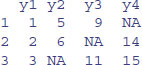
This syntax is useful in editing out rows containing missing values from large dataframes. Here is a very simple example of a dataframe with four rows and four columns:
y1 <- c(1,2,3,NA)
y2 <- c(5,6,NA,8)
y3 <- c(9,NA,11,12)
y4 <- c(NA,14,15,16)
full.frame <- data.frame(y1,y2,y3,y4)
reduced.frame <- full.frame[!is.na(full.frame$y1),]
so the new reduced.frame will have fewer rows than full.frame when the variable in full.frame called full.frame$y1 contains one or more missing values.
reduced.frame
Some functions do not work with their default settings when there are missing values in the data, and mean is a classic example of this:
x <- c(1:8,NA)
mean(x)
[1] NA
In order to calculate the mean of the non-missing values, you need to specify that the NA are to be removed, using the na.rm=TRUE argument:
mean(x,na.rm=T)
[1] 4.5
Here is an example where we want to find the locations (7 and 8) of missing values within a vector called vmv:
vmv <- c(1:6,NA,NA,9:12)
vmv
[1] 1 2 3 4 5 6 NA NA 9 10 11 12
Making an index of the missing values in an array could use the seq function, like this:
seq(along=vmv)[is.na(vmv)]
[1] 7 8
However, the result is achieved more simply using the which function like this:
which(is.na(vmv))
[1] 7 8
If the missing values are genuine counts of zero, you might want to edit the NA to 0. Use the is.na function to generate subscripts for this:
vmv[is.na(vmv)] <- 0
vmv
[1] 1 2 3 4 5 6 0 0 9 10 11 12
Or use the ifelse function like this:
vmv <- c(1:6,NA,NA,9:12)
ifelse(is.na(vmv),0,vmv)
[1] 1 2 3 4 5 6 0 0 9 10 11 12
Be very careful when doing this, because most missing values are not genuine zeros.
2.6 Vectors and subscripts
A vector is a variable with one or more values of the same type. For instance, the numbers of peas in six pods were 4, 7, 6, 5, 6 and 7. The vector called peas is one object of length = 6. In this case, the class of the object is numeric. The easiest way to create a vector in R is to concatenate (link together) the six values using the concatenate function, c, like this:
peas <- c(4, 7, 6, 5, 6, 7)
We can ask all sorts of questions about the vector called peas. For instance, what type of vector is it?
class(peas)
[1] "numeric"
How big is the vector?
length(peas)
[1] 6
The great advantage of a vector-based language is that it is very simple to ask quite involved questions that involve all of the values in the vector. These vector functions are often self-explanatory:
mean(peas)
[1] 5.833333
max(peas)
[1] 7
min(peas)
[1] 4
Others might be more opaque:
quantile(peas)
0% 25% 50% 75% 100%
4.00 5.25 6.00 6.75 7.00
Another way to create a vector is to input data from the keyboard using the function called scan:
peas <- scan()
The prompt appears 1: which means type in the first number of peas (4) then press the return key, then the prompt 2: appears (you type in 7) and so on. When you have typed in all six values, and the prompt 7: has appeared, you just press the return key to tell R that the vector is now complete. R replies by telling you how many items it has read:
1: 4
2: 7
3: 6
4: 5
5: 6
6: 7
7:
Read 6 items
For more realistic applications, the usual way of creating vectors is to read the data from a pre-prepared computer file (as described in Chapter 3).
2.6.1 Extracting elements of a vector using subscripts
You will often want to use some but not all of the contents of a vector. To do this, you need to master the use of subscripts (or indices as they are also known). In R, subscripts involve the use of square brackets []. Our vector called peas shows the numbers of peas in six pods:
peas
[1] 4 7 6 5 6 7
The first element of peas is 4, the second 7, and so on. The elements are indexed left to right, 1 to 6. It could not be more straightforward. If we want to extract the fourth element of peas (which you can see is a 5) then this is what we do:
peas[4]
[1] 5
If we want to extract several values (say the 2nd, 3rd and 6th) we use a vector to specify the pods we want as subscripts, either in two stages like this:
pods <- c(2,3,6)
peas[pods]
[1] 7 6 7
or in a single step, like this:
peas[c(2,3,6)]
[1] 7 6 7
You can drop values from a vector by using negative subscripts. Here are all but the first values of peas:
peas[-1]
[1] 7 6 5 6 7
Here are all but the last (note the use of the length function to decide what is last):
peas[-length(peas)]
[1] 4 7 6 5 6
We can use these ideas to write a function called trim to remove (say) the largest two and the smallest two values from a vector called x. First we have to sort the vector, then remove the smallest two values (these will have subscripts 1 and 2), then remove the largest two values (which will have subscripts length(x) and length(x)-1):
trim <- function(x) sort(x)[-c(1,2,length(x)-1,length(x))]
We can use trim on the vector called peas, expecting to get 6 and 6 as the result:
trim(peas)
[1] 6 6
Finally, we can use sequences of numbers to extract values from a vector. Here are the first three values of peas:
peas[1:3]
[1] 4 7 6
Here are the even-numbered values of peas:
peas[seq(2,length(peas),2)]
[1] 7 5 7
or alternatively:
peas[1:length(peas) %% 2 == 0]
[1] 7 5 7
using the modulo function %% on the sequence 1 to 6 to extract the even numbers 2, 4 and 6. Note that vectors in R could have length 0, and this could be useful in writing functions:
y <- 4.3
z <- y[-1]
length(z)
[1] 0
2.6.2 Classes of vector
The vector called peas contained numbers: in the jargon, it is of class numeric. R allows vectors of six types, so long as all of the elements in one vector belong to the same class. The classes are logical, integer, real, complex, string (or character) or raw. You will use numeric, logical and character variables all the time. Engineers and mathematicians will use complex numbers. But you could go a whole career without ever needing to use integer or raw.
2.6.3 Naming elements within vectors
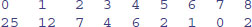
It is often useful to have the values in a vector labelled in some way. For instance, if our data are counts of 0, 1, 2, … occurrences in a vector called counts,
(counts <- c(25,12,7,4,6,2,1,0,2))
[1] 25 12 7 4 6 2 1 0 2
so that there were 25 zeros, 12 ones and so on, it would be useful to name each of the counts with the relevant number 0 to 8:
names(counts) <- 0:8
Now when we inspect the vector called counts we see both the names and the frequencies:
counts
If you have computed a table of counts, and you want to remove the names, then use the as.vector function like this:
(st <- table(rpois(2000,2.3)))

as.vector(st)
[1] 205 455 510 431 233 102 43 13 7 1
2.6.4 Working with logical subscripts
Take the example of a vector containing the 11 numbers 0 to 10:
x <- 0:10
There are two quite different kinds of things we might want to do with this. We might want to add up the values of the elements:
sum(x)
[1] 55
Alternatively, we might want to count the elements that passed some logical criterion. Suppose we wanted to know how many of the values were less than 5:
sum(x<5)
[1] 5
You see the distinction. We use the vector function sum in both cases. But sum(x) adds up the values of the xs and sum(x<5) counts up the number of cases that pass the logical condition ‘x is less than 5’. This works because of coercion (p. 30). Logical TRUE has been coerced to numeric 1 and logical FALSE has been coerced to numeric 0.
That is all well and good, but how do you add up the values of just some of the elements of x? We specify a logical condition, but we do not want to count the number of cases that pass the condition, we want to add up all the values of the cases that pass. This is the final piece of the jigsaw, and involves the use of logical subscripts. Note that when we counted the number of cases, the counting was applied to the entire vector, using sum(x<5). To find the sum of the values of x that are less than 5, we write:
sum(x[x<5])
[1] 10
Let us look at this in more detail. The logical condition x<5 is either true or false:
x<5
[1] TRUE TRUE TRUE TRUE TRUE FALSE FALSE FALSE FALSE FALSE FALSE
You can imagine false as being numeric 0 and true as being numeric 1. Then the vector of subscripts [x<5] is five 1s followed by six 0s:
1*(x<5)
[1] 1 1 1 1 1 0 0 0 0 0 0
Now imagine multiplying the values of x by the values of the logical vector
x*(x<5)
[1] 0 1 2 3 4 0 0 0 0 0 0
When the function sum is applied, it gives us the answer we want: the sum of the values of the numbers 0 + 1 + 2 + 3 + 4 = 10.
sum(x*(x<5))
[1] 10
This produces the same answer as sum(x[x<5]), but is rather less elegant.
Suppose we want to work out the sum of the three largest values in a vector. There are two steps: first sort the vector into descending order; then add up the values of the first three elements of the reverse-sorted array. Let us do this in stages. First, the values of y:
y <- c(8,3,5,7,6,6,8,9,2,3,9,4,10,4,11)
Now if you apply sort to this, the numbers will be in ascending sequence, and this makes life slightly harder for the present problem:
sort(y)
[1] 2 3 3 4 4 5 6 6 7 8 8 9
[13] 9 10 11
We can use the reverse function, rev like this (use the Up arrow key to save typing):
rev(sort(y))
[1] 11 10 9 9 8 8 7 6 6 5 4 4
[13] 3 3 2
So the answer to our problem is 11 + 10 + 9 = 30. But how to compute this? A range of subscripts is simply a series generated using the colon operator. We want the subscripts 1 to 3, so this is:
rev(sort(y))[1:3]
[1] 11 10 9
So the answer to the exercise is just:
sum(rev(sort(y))[1:3])
[1] 30
Note that we have not changed the vector y in any way, nor have we created any new space-consuming vectors during intermediate computational steps.
You will often want to find out which value in a vector is the maximum or the minimum. This is a question about indices, and the answer you want is an integer indicating which element of the vector contains the maximum (or minimum) out of all the values in that vector. Here is the vector:
x <- c(2,3,4,1,5,8,2,3,7,5,7)
So the answers we want are 6 (the maximum) and 4 (the minimum). The slow way to do it is like this:
which(x == max(x))
[1] 6
which(x == min(x))
[1] 4
Better, however, to use the much quicker built-in functions which.max or which.min like this:
which.max(x)
[1] 6
which.min(x)
[1] 4
2.7 Vector functions
One of R's great strengths is its ability to evaluate functions over entire vectors, thereby avoiding the need for loops and subscripts. The most important vector functions are listed in Table 2.4. Here is a numeric vector:
y <- c(8,3,5,7,6,6,8,9,2,3,9,4,10,4,11)
Some vector functions produce a single number:
mean(y)
[1] 6.333333
Others produce two numbers:
range(y)
[1] 2 11
here showing that the minimum was 2 and the maximum was 11. Other functions produce several numbers:
fivenum(y)
[1] 2.0 4.0 6.0 8.5 11.0
This is Tukey's famous five-number summary: the minimum, the lower hinge, the median, the upper hinge and the maximum (the hinges are explained on p. 346).
Perhaps the single most useful vector function in R is table. You need to see it in action to appreciate just how good it is. Here is a huge vector called counts containing 10 000 random integers from a negative binomial distribution (counts of fungal lesions on 10 000 individual leaves, for instance):
counts <- rnbinom(10000,mu=0.92,size=1.1)
Here is a look at the first 30 values in counts:
counts[1:30]
[1] 3 1 0 0 1 0 0 0 0 1 1 0 0 2 0 1 3 1 0 1 0 1 1 0 0 2 1 4 0 1
The question is this: how many zeros are there in the whole vector of 10 000 numbers, how many 1s, and so on right up to the largest value within counts? A formidable task for you or me, but for R it is just:
table(counts)
counts
0 1 2 3 4 5 6 7 8 9 10 11 13
5039 2574 1240 607 291 141 54 29 11 9 3 1 1
There were 5039 zeros, 2574 ones, and so on up the largest counts (there was one 11 and one 13 in this realization; you will have obtained different random numbers on your computer).
Table 2.4 Vector functions used in R.
| Operation | Meaning |
| max(x) | maximum value in x |
| min(x) | minimum value in x |
| sum(x) | total of all the values in x |
| mean(x) | arithmetic average of the values in x |
| median(x) | median value in x |
| range(x) | vector of min(x) and max(x) |
| var(x) | sample variance of x |
| cor(x,y) | correlation between vectors x and y |
| sort(x) | a sorted version of x |
| rank(x) | vector of the ranks of the values in x |
| order(x) | an integer vector containing the permutation to sort x into ascending order |
| quantile(x) | vector containing the minimum, lower quartile, median, upper quartile, and maximum of x |
| cumsum(x) | vector containing the sum of all of the elements up to that point |
| cumprod(x) | vector containing the product of all of the elements up to that point |
| cummax(x) | vector of non-decreasing numbers which are the cumulative maxima of the values in x up to that point |
| cummin(x) | vector of non-increasing numbers which are the cumulative minima of the values in x up to that point |
| pmax(x,y,z) | vector, of length equal to the longest of x, y or z, containing the maximum of x, y or z for the ith position in each |
| pmin(x,y,z) | vector, of length equal to the longest of x, y or z, containing the minimum of x, y or z for the ith position in each |
| colMeans(x) | column means of dataframe or matrix x |
| colSums(x) | column totals of dataframe or matrix x |
| rowMeans(x) | row means of dataframe or matrix x |
| rowSums(x) | row totals of dataframe or matrix x |
2.7.1 Obtaining tables of means using tapply
One of the most important functions in all of R is tapply. It does not sound like much from the name, but you will use it time and again for calculating means, variances, sample sizes, minima and maxima. With weather data, for instance, we might want the 12 monthly mean temperatures rather than the whole-year average. We have a response variable, temperature, and a categorical explanatory variable, month:
data<-read.table("c:\\temp\\temperatures.txt",header=T)
attach(data)
names(data)
[1] "temperature" "lower" "rain" "month" "yr"
The function that we want to apply is mean. All we do is invoke the tapply function with three arguments: the response variable, the categorical explanatory variable and the name of the function that we want to apply:
tapply(temperature,month,mean)
It is easy to apply other functions in the same way: here are the monthly variances
tapply(temperature,month,var)
and the monthly minima
tapply(temperature,month,min)
If R does not have a built in function to do what you want (Table 2.4), then you can easily write your own. Here, for instance, is a function to calculate the standard error of each mean (these are called anonymous functions in R, because they are unnamed):
tapply(temperature,month,function(x) sqrt(var(x)/length(x)))
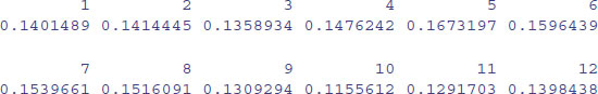
The tapply function is very flexible. It can produce multi-dimensional tables simply by replacing the one categorical variable (month) by a list of categorical variables. Here are the monthly means calculated separately for each year, as specified by list(yr,month). The variable you name first in the list (yr) will appear as the row of the results table and the second will appear as the columns (month):
tapply(temperature,list(yr,month),mean)[,1:6]
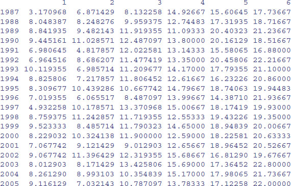
The subscripts [,1:6] simply restrict the output to the first six months. You can see at once that January (month 1) 1993 was exceptionally warm and January 1987 exceptionally cold.
There is just one thing about tapply that might confuse you. If you try to apply a function that has built-in protection against missing values, then tapply may not do what you want, producing NA instead of the numerical answer. This is most likely to happen with the mean function because its default is to produce NA when there are one or more missing values. The remedy is to provide an extra argument to tapply, specifying that you want to see the average of the non-missing values. Use na.rm=TRUE to remove the missing values like this:
tapply(temperature,yr,mean,na.rm=TRUE)
You might want to trim some of the extreme values before calculating the mean (the arithmetic mean is famously sensitive to outliers). The trim option allows you to specify the fraction of the data (between 0 and 0.5) that you want to be omitted from the left- and right-hand tails of the sorted vector of values before computing the mean of the central values:
tapply(temperature,yr,mean,trim=0.2)

2.7.2 The aggregate function for grouped summary statistics
Suppose that we have two response variables (y and z) and two explanatory variables (x and w) that we might want to use to summarize functions like mean or variance of y and/or z. The aggregate function has a formula method which allows elegant summaries of four kinds:
| one to one | aggregate(y ~ x, mean) |
| one to many | aggregate(y ~ x + w, mean) |
| many to one | aggregate(cbind(y,z) ~ x, mean) |
| many to many | aggregate(cbind(y,z) ~ x + w, mean) |
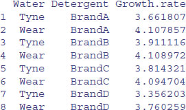
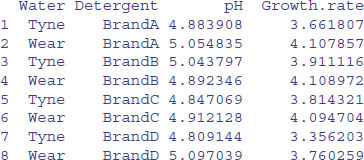
This is very useful for removing pseudoreplication from dataframes. Here is an example using a dataframe with two continuous variables (Growth.rate and pH) and three categorical explanatory variables (Water, Detergent and Daphnia):
data<-read.table("c:\\temp\\pHDaphnia.txt",header=T)
names(data)
[1] "Growth.rate" "Water" "Detergent" "Daphnia" "pH"
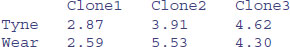
Here is one-to-one use of aggregate to find mean growth rate in the two water samples:
aggregate(Growth.rate~Water,data,mean)
Water Growth.rate
1 Tyne 3.685862
2 Wear 4.017948
Here is a one-to-many use to look at the interaction between Water and Detergent:
aggregate(Growth.rate~Water+Detergent,data,mean)
Finally, here is a many-to-many use to find mean pH as well as mean Growth.rate for the interaction between Water and Detergent:
aggregate(cbind(pH,Growth.rate)~Water+Detergent,data,mean)
2.7.3 Parallel minima and maxima: pmin and pmax
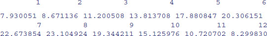
Here are three vectors of the same length, x, y and z. The parallel minimum function, pmin, finds the minimum from any one of the three variables for each subscript, and produces a vector as its result (of length equal to the longest of x, y, or z):
x
[1] 0.99822644 0.98204599 0.20206455 0.65995552 0.93456667 0.18836278
y
[1] 0.51827913 0.30125005 0.41676059 0.53641449 0.07878714 0.49959328
z
[1] 0.26591817 0.13271847 0.44062782 0.65120395 0.03183403 0.36938092
pmin(x,y,z)
[1] 0.26591817 0.13271847 0.20206455 0.53641449 0.03183403 0.18836278
Thus the first and second minima came from z, the third from x, the fourth from y, the fifth from z, and the sixth from x. The functions min and max produce scalar results, not vectors.
2.7.4 Summary information from vectors by groups
The vector function tapply is one of the most important and useful vector functions to master. The ‘t’ stands for ‘table’ and the idea is to apply a function to produce a table from the values in the vector, based on one or more grouping variables (often the grouping is by factor levels). This sounds much more complicated than it really is:
data <- read.table("c:\\temp\\daphnia.txt",header=T)
attach(data)
names(data)
[1] "Growth.rate" "Water" "Detergent" "Daphnia"
The response variable is Growth.rate and the other three variables are factors (the analysis is on p. 528). Suppose we want the mean growth rate for each detergent:
tapply(Growth.rate,Detergent,mean)

This produces a table with four entries, one for each level of the factor called Detergent. To produce a two-dimensional table we put the two grouping variables in a list. Here we calculate the median growth rate for water type and daphnia clone:
tapply(Growth.rate,list(Water,Daphnia),median)
The first variable in the list creates the rows of the table and the second the columns. More detail on the tapply function is given in Chapter 6 (p. 245).
2.7.5 Addresses within vectors
There is an important function called which for finding addresses within vectors. The vector y looks like this:
y <- c(8,3,5,7,6,6,8,9,2,3,9,4,10,4,11)
Suppose we wanted to know which elements of y contained values bigger than 5. We type:
which(y>5)
[1] 1 4 5 6 7 8 11 13 15
Notice that the answer to this enquiry is a set of subscripts. We do not use subscripts inside the which function itself. The function is applied to the whole array. To see the values of y that are larger than 5, we just type:
y[y>5]
[1] 8 7 6 6 8 9 9 10 11
Note that this is a shorter vector than y itself, because values of 5 or less have been left out:
length(y)
[1] 15
length(y[y>5])
[1] 9
2.7.6 Finding closest values
Finding the value in a vector that is closest to a specified value is straightforward using which. The vector xv contains 1000 random numbers from a normal distribution with mean = 100 and standard deviation = 10:
xv <- rnorm(1000,100,10)
Here, we want to find the value of xv that is closest to 108.0. The logic is to work out the difference between 108 and each of the 1000 random numbers, then find which of these differences is the smallest. This is what the R code looks like:
which(abs(xv-108)==min(abs(xv-108)))
[1] 332
The closest value to 108.0 is in location 332 within xv. But just how close to 108.0 is this 332nd value? We use 332 as a subscript on xv to find this out:
xv[332]
[1] 108.0076
Now we can write a function to return the closest value to a specified value (sv) in any vector (xv):
closest <- function(xv,sv){
xv[which(abs(xv-sv)==min(abs(xv-sv)))] }
and run it like this:
closest(xv,108)
[1] 108.0076
2.7.7 Sorting, ranking and ordering
These three related concepts are important, and one of them (order) is difficult to understand on first acquaintance. Let us take a simple example:
houses <- read.table("c:\\temp\\houses.txt",header=T)
attach(houses)
names(houses)
[1] "Location" "Price"
We apply the three different functions to the vector called Price:
ranks <- rank(Price)
sorted <- sort(Price)
ordered <- order(Price)
Then we make a dataframe out of the four vectors like this:
view <- data.frame(Price,ranks,sorted,ordered)
view
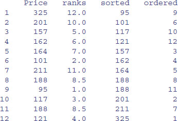
Rank
The prices themselves are in no particular sequence. The ranks column contains the value that is the rank of the particular data point (value of Price), where 1 is assigned to the lowest data point and length(Price) – here 12 – is assigned to the highest data point. So the first element, a price of 325, happens to be the highest value in Price. You should check that there are 11 values smaller than 325 in the vector called Price. Fractional ranks indicate ties. There are two 188s in Price and their ranks are 8 and 9. Because they are tied, each gets the average of their two ranks (8 + 9)/2 = 8.5. The lowest price is 95, indicated by a rank of 1.
Sort
The sorted vector is very straightforward. It contains the values ofPrice sorted into ascending order. If you want to sort into descending order, use the reverse order function rev like this:
y <- rev(sort(x))
Note that sort is potentially very dangerous, because it uncouples values that might need to be in the same row of the dataframe (e.g. because they are the explanatory variables associated with a particular value of the response variable). It is bad practice, therefore, to write x <- sort(x), not least because there is no ‘unsort’ function.
Order
This is the most important of the three functions, and much the hardest to understand on first acquaintance. The numbers in this column are subscripts between 1 and 12. The order function returns an integer vector containing the permutation that will sort the input into ascending order. You will need to think about this one. The lowest value of Price is 95. Look at the dataframe and ask yourself what is the subscript in the original vector called Price where 95 occurred. Scanning down the column, you find it in row number 9. This is the first value in ordered, ordered[1]. Where is the next smallest value (101) to be found within Price? It is in position 6, so this is ordered[2]. The third smallest value of Price (117) is in position 10, so this is ordered[3]. And so on.
This function is particularly useful in sorting dataframes, as explained on p. 166. Using order with subscripts is a much safer option than using sort, because with sort the values of the response variable and the explanatory variables could be uncoupled with potentially disastrous results if this is not realized at the time that modelling was carried out. The beauty of order is that we can use order(Price) as a subscript for Location to obtain the price-ranked list of locations:
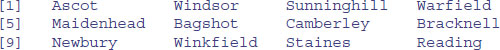
Location[order(Price)]

When you see it used like this, you can see exactly why the function is called order. If you want to reverse the order, just use the rev function like this:
Location[rev(order(Price))]
Make sure you understand why some of the brackets are round and some are square.
2.7.8 Understanding the difference between unique and duplicated
The difference is best seen with a simple example. Here is a vector of names:
names <- c("Williams","Jones","Smith","Williams","Jones","Williams")
We can see how many times each name appears using table:
table(names)
names
Jones Smith Williams
2 1 3
It is clear that the vector contains just three different names. The function called unique extracts these three unique names, creating a vector of length 3, unsorted, in the order in which the names are encountered in the vector:
unique(names)
[1] "Williams" "Jones" "Smith"
In contrast, the function called duplicated produces a vector, of the same length as the vector of names, containing the logical values either FALSE or TRUE, depending upon whether or not that name has appeared already (reading from the left). You need to see this in action to understand what is happening, and why it might be useful:
duplicated(names)
[1] FALSE FALSE FALSE TRUE TRUE TRUE
The first three names are not duplicated (FALSE), but the last three are all duplicated (TRUE). We can mimic the unique function by using this vector as subscripts like this:
names[!duplicated(names)]
[1] "Williams" "Jones" "Smith"
Note the use of the NOT operator (!) in front of the duplicated function. There you have it: if you want a shortened vector, containing only the unique values in names, then use unique, but if you want a vector of the same length as names then use duplicated. You might use this to extract values from a different vector (salaries, for instance) if you wanted the mean salary, ignoring the repeats:
salary <- c(42,42,48,42,42,42)
mean(salary)
[1] 43
salary[!duplicated(names)]
[1] 42 42 48
mean(salary[!duplicated(names)])
[1] 44
Note that this is not the same answer as would be obtained by omitting the duplicate salaries, because two of the people (Jones and Williams) had the same salary (42). Here is the wrong answer:
mean(salary[!duplicated(salary)])
[1] 45
2.7.9 Looking for runs of numbers within vectors
The function called rle, which stands for ‘run length encoding’ is most easily understood with an example. Here is a vector of 150 random numbers from a Poisson distribution with mean 0.7:
(poisson <- rpois(150,0.7))
[1] 1 1 0 0 2 1 0 1 0 0 1 1 1 0 1 1 2 1 1 0 1 0 2 1 1 2 0 2 0 1 0 0 0 2 0
[36] 1 0 4 0 0 1 0 1 0 1 0 2 1 1 1 0 1 0 1 0 0 0 0 0 0 0 2 0 0 0 0 1 0 0 0
[71] 2 1 1 1 1 0 1 0 1 0 0 1 1 0 1 0 2 1 1 2 0 1 0 1 0 0 0 1 1 0 1 2 2 0 1
[106] 0 0 0 0 0 0 1 0 0 2 1 2 0 2 0 2 2 1 1 0 2 0 1 1 2 2 2 1 1 1 1 0 0 0 1
[141] 0 2 1 4 0 0 2 1 0 1
We can do our own run length encoding on the vector by eye: there is a run of two 1s, then a run of two 0s, then a single 2, then a single 1, then a single 0, and so on. So the run lengths are 2, 2, 1, 1, 1, 1, …. The values associated with these runs were 1, 0, 2, 1, 0, 1, …. Here is the output from rle:
rle(poisson)
Run Length Encoding
lengths: int [1:93] 2 2 1 2 1 1 2 3 1 2 1 …
values : num [1:93] 1 0 2 1 0 1 0 1 2 1 …
The object produced by rle is a list of two vectors: the lengths of the runs and the values that did the running. To find the longest run, and the value associated with that longest run, we use the indexed lists like this:
max(rle(poisson)[[1]])
[1] 7
So the longest run in this vector of numbers was 7. But 7 of what? We use which to find the location of the 7 in lengths, then apply this index to values to find the answer:
which(rle(poisson)[[1]]==7)
[1] 55
rle(poisson)[[2]][55]
[1] 0
So, not surprisingly given that the mean was just 0.7, the longest run was of zeros.
Here is a function to return the length of the run and its value for any vector:
run.and.value <- function (x) {
a <- max(rle(poisson)[[1]])
b <- rle(poisson)[[2]][which(rle(poisson)[[1]] == a)]
cat("length = ",a," value = ",b, "\n")}
Testing the function on the vector of 150 Poisson data gives:
run.and.value(poisson)
length = 7 value = 0
It is sometimes of interest to know the number of runs in a given vector (for instance, the lower the number of runs, the more aggregated the numbers; and the greater the number of runs, the more regularly spaced out). We use the length function for this:
length(rle(poisson)[[2]])
[1] 93
indicating that the 150 values were arranged in 93 runs (this is an intermediate value, characteristic of a random pattern). The value 93 appears in square brackets [1:93] in the output of the run length encoding function.
In a different example, suppose we had n1 values of 1 representing ‘present’ and n2 values of 0 representing ‘absent’; then the minimum number of runs would be 2 (a solid block of 1s then a sold block of 0s). The maximum number of runs would be 2n + 1 if they alternated (until the smaller number n = min(n1,n2) ran out). Here is a simple runs test based on 1000 randomizations of 25 ones and 30 zeros:
n1 <- 25
n2 <- 30
y <- c(rep(1,n1),rep(0,n2))
len <- numeric(10000)
for (i in 1:10000) len[i] <- length(rle(sample(y))[[2]])
quantile(len,c(0.025,0.975))
2.5% 97.5%
21 35
Thus, for these data (n1 = 25 and n2 = 30) an aggregated pattern would score 21 or fewer runs, and a regular pattern would score 35 or more runs. Any scores between 21 and 35 fall within the realm of random patterns.
2.7.10 Sets: union, intersect and setdiff
There are three essential functions for manipulating sets. The principles are easy to see if we work with an example of two sets:
setA <- c("a", "b", "c", "d", "e")
setB <- c("d", "e", "f", "g")
Make a mental note of what the two sets have in common, and what is unique to each.
The union of two sets is everything in the two sets taken together, but counting elements only once that are common to both sets:
union(setA,setB)
[1] "a" "b" "c" "d" "e" "f" "g"
The intersection of two sets is the material that they have in common:
intersect(setA,setB)
[1] "d" "e"
Note, however, that the difference between two sets is order-dependent. It is the material that is in the first named set, that is not in the second named set. Thus setdiff(A,B) gives a different answer than setdiff(B,A). For our example:
setdiff(setA,setB)
[1] "a" "b" "c"
setdiff(setB,setA)
[1] "f" "g"
Thus, it should be the case that setdiff(setA,setB) plus intersect(setA,setB) plus setdiff(setB,setA) is the same as the union of the two sets. Let us check:
all(c(setdiff(setA,setB),intersect(setA,setB),setdiff(setB,setA))==
union(setA,setB))
[1] TRUE
There is also a built-in function setequal for testing if two sets are equal:
setequal(c(setdiff(setA,setB),intersect(setA,setB),setdiff(setB,setA)),
union(setA,setB))
[1] TRUE
You can use %in% for comparing sets. The result is a logical vector whose length matches the vector on the left:
setA %in% setB
[1] FALSE FALSE FALSE TRUE TRUE
setB %in% setA
[1] TRUE TRUE FALSE FALSE
Using these vectors of logical values as subscripts, we can demonstrate, for instance, that setA[setA %in% setB] is the same as intersect(setA,setB):
setA[setA %in% setB]
[1] "d" "e"
intersect(setA,setB)
[1] "d" "e"
2.8 Matrices and arrays
An array is a multi-dimensional object. The dimensions of an array are specified by its dim attribute, which gives the maximal indices in each dimension. So for a three-dimensional array consisting of 24 numbers in a sequence 1:24, with dimensions 2 × 4 × 3, we write:
y <- 1:24
dim(y) <- c(2,4,3)
y
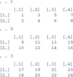
This produces three two-dimensional tables, because the third dimension is 3. This is what happens when you change the dimensions:
dim(y) <- c(3,2,4)
y
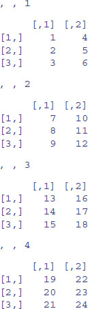
Now we have four two-dimensional tables, each of three rows and two columns. Keep looking at these two examples until you are sure that you understand exactly what has happened here.
A matrix is a two-dimensional array containing numbers. A dataframe is a two-dimensional list containing (potentially a mix of) numbers, text or logical variables in different columns. When there are two subscripts [5,3] to an object like a matrix or a dataframe, the first subscript refers to the row number (5 in this example; the rows are defined as margin number 1) and the second subscript refers to the column number (3 in this example; the columns are margin number 2). There is an important and powerful convention in R, such that when a subscript appears as a blank it is understood to mean ‘all of’. Thus:
- [,4] means all rows in column 4 of an object;
- [2,] means all columns in row 2 of an object.
2.8.1 Matrices
There are several ways of making a matrix. You can create one directly like this:
X <- matrix(c(1,0,0,0,1,0,0,0,1),nrow=3)
X
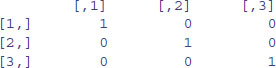
where, by default, the numbers are entered column-wise. The class and attributes of X indicate that it is a matrix of three rows and three columns (these are its dim attributes):
class(X)
[1] "matrix"
attributes(X)
$dim
[1] 3 3
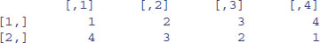
In the next example, the data in the vector appear row-wise, so we indicate this with byrow=T:
vector <- c(1,2,3,4,4,3,2,1)
V <- matrix(vector,byrow=T,nrow=2)
V

Another way to convert a vector into a matrix is by providing the vector object with two dimensions (rows and columns) using the dim function like this:
dim(vector) <- c(4,2)
We can check that vector has now become a matrix:
is.matrix(vector)
[1] TRUE
We need to be careful, however, because we have made no allowance at this stage for the fact that the data were entered row-wise into vector:
vector
[,1] [,2]
[1,] 1 4
[2,] 2 3
[3,] 3 2
[4,] 4 1
The matrix we want is the transpose, t, of this matrix:
(vector <- t(vector))
2.8.2 Naming the rows and columns of matrices
At first, matrices have numbers naming their rows and columns (see above). Here is a 4 × 5 matrix of random integers from a Poisson distribution with mean 1.5:
X <- matrix(rpois(20,1.5),nrow=4)
X
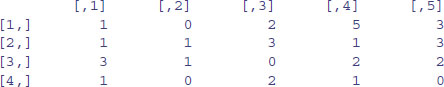
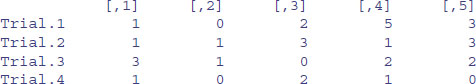
Suppose that the rows refer to four different trials and we want to label the rows ‘Trial.1’ etc. We employ the function rownames to do this. We could use the paste function (see p. 87) but here we take advantage of the prefix option:
rownames(X) <- rownames(X,do.NULL=FALSE,prefix="Trial.")
X
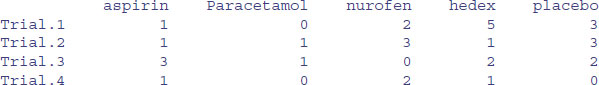
For the columns we want to supply a vector of different names for the five drugs involved in the trial, and use this to specify the colnames(X):
drug.names <- c("aspirin", "paracetamol", "nurofen", "hedex", "placebo")
colnames(X) <- drug.names
X
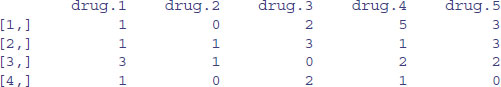
Alternatively, you can use the dimnames function to give names to the rows and/or columns of a matrix. In this example we want the rows to be unlabelled (NULL) and the column names to be of the form ‘drug.1’, ‘drug.2’, etc. The argument to dimnames has to be a list (rows first, columns second, as usual) with the elements of the list of exactly the correct lengths (4 and 5 in this particular case):
dimnames(X) <- list(NULL,paste("drug.",1:5,sep=""))
X
2.8.3 Calculations on rows or columns of the matrix
We could use subscripts to select parts of the matrix, with a blank meaning ‘all of the rows’ or ‘all of the columns’. Here is the mean of the rightmost column (number 5), calculated over all the rows (blank then comma),
mean(X[,5])
[1] 2
or the variance of the bottom row, calculated over all of the columns (a blank in the second position),
var(X[4,])
[1] 0.7
There are some special functions for calculating summary statistics on matrices:
rowSums(X)
[1] 11 9 8 4
colSums(X)
[1] 6 2 7 9 8
rowMeans(X)
[1] 2.2 1.8 1.6 0.8
colMeans(X)
[1] 1.50 0.50 1.75 2.25 2.00
These functions are built for speed, and blur some of the subtleties of dealing with NA or NaN. If such subtlety is an issue, then use apply instead (p. 61). Remember that columns are margin number 2 and rows are margin number 1:
apply(X,2,mean)
[1] 1.50 0.50 1.75 2.25 2.00
You might want to sum groups of rows within columns, and rowsum (singular and all lower case, in contrast to rowSums, above) is a very efficient function for this. In this example, we want to group together row 1 and row 4 (as group A) and row 2 and row 3 (group B). Note that the grouping vector has to have length equal to the number of rows:
group=c("A","B","B","A")
rowsum(X, group)
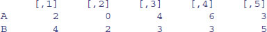
You could achieve the same ends (but more slowly) with tapply or aggregate:
tapply(X, list(group[row(X)], col(X)), sum)
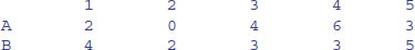
Note the use of row(X) and col(X), with row(X) used as a subscript on group.
aggregate(X,list(group),sum)
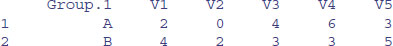
Suppose that we want to shuffle the elements of each column of a matrix independently. We apply the function sample to each column (margin number 2) like this:
apply(X,2,sample)
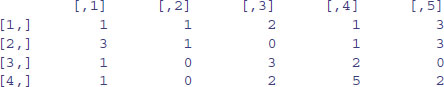
apply(X,2,sample)
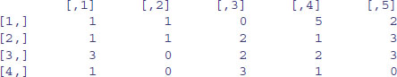
and so on, for as many shuffled samples as you need.
2.8.4 Adding rows and columns to the matrix
In this particular case we have been asked to add a row at the bottom showing the column means, and a column at the right showing the row variances:
X <- rbind(X,apply(X,2,mean))
X <- cbind(X,apply(X,1,var))
X
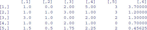
Note that the number of decimal places varies across columns, with one in columns 1 and 2, two in columns 3 and 4, none in column 5 (integers) and five in column 6. The default in R is to print the minimum number of decimal places consistent with the contents of the column as a whole.
Next, we need to label the sixth column as ‘variance’ and the fifth row as ‘mean’:
colnames(X) <- c(1:5,"variance")
rownames(X) <- c(1:4,"mean")
X
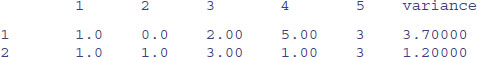

When a matrix with a single row or column is created by a subscripting operation, for example row <- mat[2,], it is by default turned into a vector. In a similar way, if an array with dimension, say, 2 × 3 × 1 × 4 is created by subscripting it will be coerced into a 2 × 3 × 4 array, losing the unnecessary dimension. After much discussion this has been determined to be a feature of R. To prevent this happening, add the option drop = FALSE to the subscripting. For example:
rowmatrix <- mat[2, , drop = FALSE]
colmatrix <- mat[, 2, drop = FALSE]
a <- b[1, 1, 1, drop = FALSE]
The drop = FALSE option should be used defensively when programming. For example, the statement
somerows <- mat[index,]
will return a vector rather than a matrix if index happens to have length 1, and this might cause errors later in the code. It should be written as:
somerows <- mat[index , , drop = FALSE]
2.8.5 The sweep function
The sweep function is used to ‘sweep out’ array summaries from vectors, matrices, arrays or dataframes. In this example we want to express a matrix in terms of the departures of each value from its column mean.
matdata <- read.table("c: \\temp \\sweepdata.txt")
First, you need to create a vector containing the parameters that you intend to sweep out of the matrix. In this case we want to compute the four column means:
(cols <- apply(matdata,2,mean))

Now it is straightforward to express all of the data in matdata as departures from the relevant column means:
sweep(matdata,2,cols)
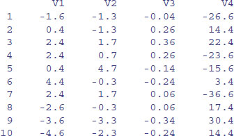
Note the use of margin = 2 as the second argument to indicate that we want the sweep to be carried out on the columns (rather than on the rows). A related function, scale, is used for centring and scaling data in terms of standard deviations (p. 254).
You can see what sweep has done by doing the calculation long-hand. The operation of this particular sweep is simply one of subtraction. The only issue is that the subtracted object has to have the same dimensions as the matrix to be swept (in this example, 10 rows of 4 columns). Thus, to sweep out the column means, the object to be subtracted from matdata must have the each column mean repeated in each of the 10 rows of 4 columns:
(col.means <- matrix(rep(cols,rep(10,4)),nrow=10))
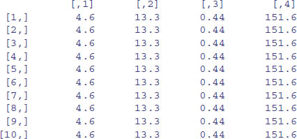
Then the same result as we got from sweep is obtained simply by
matdata-col.means
Suppose that you want to obtain the subscripts for a column-wise or a row-wise sweep of the data. Here are the row subscripts repeated in each column:
apply(matdata,2,function (x) 1:10)
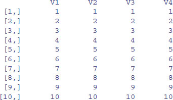
Here are the column subscripts repeated in each row:
t(apply(matdata,1,function (x) 1:4))
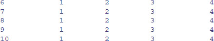
Here is the same procedure using sweep:
sweep(matdata,1,1:10,function(a,b) b)
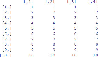
sweep(matdata,2,1:4,function(a,b) b)
2.8.6 Applying functions with apply, sapply and lapply
The apply function is used for applying functions to the rows or columns of matrices or dataframes. For example, here is a matrix with four rows and six columns:
(X <- matrix(1:24,nrow=4))
Note that placing the expression to be evaluated in parentheses (as above) causes the value of the result to be printed on the screen. Often you want to apply a function across one of the margins of a matrix. Margin 1 refers to the rows and margin 2 to the columns. Here are the row totals (four of them):
apply(X,1,sum)
[1] 66 72 78 84
and here are the column totals (six of them):
apply(X,2,sum)
[1] 10 26 42 58 74 90
Note that in both cases, the answer produced by apply is a vector rather than a matrix. You can apply functions to the individual elements of the matrix rather than to the margins. The margin you specify influences only the shape of the resulting matrix.
apply(X,1,sqrt)
apply(X,2,sqrt)
Here are the shuffled numbers from each of the rows, using sample without replacement:
apply(X,1,sample)
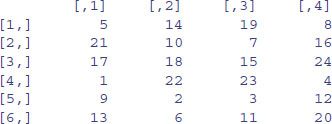
Note that the resulting matrix has six rows and four columns (i.e. it has been transposed).
You can supply your own function definition (here x2 + x) within apply like this:
apply(X,1,function(x) x^ 2+x)
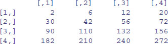

This is an anonymous function because the function is not named.
If you want to apply a function to a vector (rather than to the margin of a matrix) then use sapply . Here is the code to generate a list of sequences from 1:3 up to 1:7 (see p. 30):
sapply(3:7, seq)

The function sapply is most useful with complicated iterative calculations. The following data show decay of radioactive emissions over a 50-day period, and we intend to use non-linear least squares (see p. 715) to estimate the decay rate a in y = exp(–ax):
sapdecay <- read.table("c:\\temp\\sapdecay.txt",header=T)
attach(sapdecay)
names(sapdecay)
[1] "x" "y"
We need to write a function to calculate the sum of the squares of the differences between the observed (y) and predicted (yf) values of y, when provided with a specific value of the parameter a:
sumsq <- function(a,xv=x,yv=y)
{ yf <- exp(-a*xv)
sum((yv-yf)^2) }
We can get a rough idea of the decay constant, a, for these data by linear regression of log(y) against x, like this:
lm(log(y)~x)
Coefficients:
(Intercept) x
0.04688 -0.05849
So our parameter a is somewhere close to 0.058. We generate a range of values for a spanning an interval on either side of 0.058:
a <- seq(0.01,0.2,.005)
Now we can use sapply to apply the sum of squares function for each of these values of a (without writing a loop), and plot the deviance against the parameter value for a:
plot(a,sapply(a,sumsq),type="l")
This shows that the least-squares estimate of a is indeed close to 0.06 (this is the value of a associated with the minimum deviance). To extract the minimum value of a we use min with subscripts (square brackets):
a[min(sapply(a,sumsq))==sapply(a,sumsq)]
[1] 0.055
Finally, we could use this value of a to generate a smooth exponential function to fit through our scatter of data points:
plot(x,y)
xv <- seq(0,50,0.1)
lines(xv,exp(-0.055*xv))
Here is the same procedure streamlined by using the optimize function. Write a function showing how the sum of squares depends on the value of the parameter a:
fa <- function(a) sum((y-exp(-a*x))^2)
Now use optimize with a specified range of values for a, here c(0.01,0.1), to find the value of a that minimizes the sum of squares:
optimize(fa,c(0.01,0.1))
$minimum
[1] 0.05538411
$objective
[1] 0.01473559
The value of a is that minimizes the sum of squares is 0.055 38 and the minimum value of the sum of squares is 0.0147.
What if we had chosen a different way of assessing the fit of the model to the data? Instead of minimizing the sum of the squares of the residuals, we might want to minimize the sum of the absolute values of the residuals. We need to write a new function to calculate this quantity:
fb <- function(a) sum(abs(y-exp(-a*x)))
Then we use optimize as before:
optimize(fb,c(0.01,0.1))
$minimum
[1] 0.05596058
$objective
[1] 0.3939221
The results differ only in the fourth digit after the decimal point, and you could not choose between the two methods from a plot of the model. Sums of squares are not the only way of doing statistics, just the conventional way.
2.8.7 Using the max.col function
The task is to work out the number of plots on which a species is dominant in the Park Grass dataframe. This involves scanning each row of a matrix and reporting on the column number that contains the maximum value.
data <- read.table("c:\\temp\\pgfull.txt",header=T)
attach(data)
names(data)
The species names are represented by two-letter codes (so, for example, ‘AC’ is Agrostis capillaris). We define the dominant as the species that has the maximum biomass on a given plot. The first task is to create a dataframe that contains only the species abundances (we do not want the plot numbers, or the treatments, or the values of any covariates). For the Park Grass data, the first 54 columns contain species abundance values, so we select all of the rows in the first 54 columns like this:
species <- data[,1:54]
Now we use the function max.col to go through all of the 89 rows, and for each row return the column number that contains the maximum biomass:
max.col(species)

To get the identity of the dominant, we then extract the name of this column, using the index returned by max.col as a subscript to the object called names(species):
names(species)[max.col(species)]
Finally, we use table to count up the total number of plots on which each species was dominant. The code looks like this:
table(names(species)[max.col(species)])
AC AE AO AP CN FR HL HS LH LP TP
26 23 4 2 1 19 3 1 5 1 4
So AC was dominant on more plots than any other species, with AE in second place and FR in third. The total number of species that were dominant on one or more plots is given by determining the length of this table:
length(table(names(species)[max.col(species)]))
[1] 11
So the number of species that were present in the system, but never attained dominance was
54 − 11 = 43:
length(names(species))-length(table(names(species)[max.col(species)]))
[1] 43
There is no such function as ‘min.col’, but you can easily emulate it by using max.col with the negatives of your data. It makes no sense to do it with this example, because several species are absent from every plot, and the function would just pick one of the absent species at random. But, anyway,
max.col(-species)
picks out the identity (the column number) of one of the zeros from each row of the dataframe. In a case where there was a unique minimum in each row, then this would find it.
2.8.8 Restructuring a multi-dimensional array using aperm
There are circumstances where you may want to reorder the dimensions of an array. Here is an example of an array with three dimensions: two sexes, three ages and four income groups. For simplicity and ease of illustration the values in the array are just the numbers 1 to 24 in order (2 × 3 × 4 = 24):
data <- array(1:24, 2:4)
The second argument to the array function specifies the number of levels in dimensions 1, 2, and 3 using the sequence-generator 2:4 to produce the numbers 2, 3 and 4. This is what the array looks like:
data
There are four sub-tables, each with 2 rows and 3 columns. Now we give names to the factor levels in each of the three dimensions: these are called the dimnames attributes and are allocated as lists like this:
dimnames(data)[[1]] <- list("male","female")
dimnames(data)[[2]] <- list("young","mid","old")
dimnames(data)[[3]] <- list("A","B","C","D")
dimnames(data)
[[1]]
[1] "male" "female"
[[2]]
[1] "young" "mid" "old"
[[3]]
[1] "A" "B" "C" "D"
You can see the advantage of naming the dimensions by comparing the output of the array with (below) and without names (above):
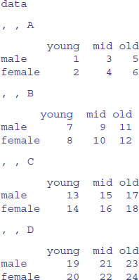
Suppose, however, that we want the four income groups (A--D) to be the columns in each of the sub-tables, and the separate sub-tables to represent the two genders. This is a job for aperm. We need to specify the order ‘age then income then gender’ in terms of the order of their dimensions (row, column, sub-table, namely 2 then 3 then 1) like this:
new.data <- aperm(data,c(2,3,1))
new.data
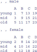
This will be tricky to see at first, but you should persevere, because aperm is a very useful function.
2.9 Random numbers, sampling and shuffling
When debugging a program it is often useful to be able to get the same string of random numbers as you had last time. Use the set.seed function to control this:
set.seed(375)
runif(3)
[1] 0.9613669 0.6918535 0.7302684
runif(3)
[1] 0.9228566 0.1603804 0.9642799
runif(3)
[1] 0.52880907 0.08660864 0.29075809
If you reset the seed with the same value, you get the same random numbers as last time:
set.seed(375)
runif(3)
[1] 0.9613669 0.6918535 0.7302684
You might want to obtain part of the same series of random numbers, and we use .Random.seed like this:
current<-.Random.seed
runif(3)
[1] 0.9228566 0.1603804 0.9642799
runif(3)
[1] 0.52880907 0.08660864 0.29075809
runif(3)
[1] 0.02590182 0.85520652 0.31350305
Resetting .Random.seed recreates the same series of random numbers:
.Random.seed<-current
runif(3)
[1] 0.9228566 0.1603804 0.9642799
Randomization is central to a great many scientific and statistical procedures. Generating random numbers from a variety of probability distributions is explained in Chapter 7 (p. 272). Here we are concerned with randomizing (shuffling or sampling from) the elements of a vector, as we might use when planning a designed experiment (e.g. allocating treatments to individuals). There are two ways of sampling:
- sampling without replacement (where all of the values in the vector appear in the output, but in a randomized sequence; i.e. the values have been shuffled);
- sampling with replacement (where some values are omitted, and other values appear more than once in the output).
2.9.1 The sample function
The default sample function shuffles the contents of a vector into a random sequence while maintaining all the numerical values intact. It is extremely useful for randomization in experimental design, in simulation and in computationally intensive hypothesis testing. The vector y looks like this:
y <- c(8,3,5,7,6,6,8,9,2,3,9,4,10,4,11)
Here are two different shufflings of y:
sample(y)

sample(y)

The order of the values is different each time sample is invoked, but the same numbers are shuffled in every case, and all the numbers in the original vector appear once in the output (so if there are two 9s in the original data, there will be two 9s in the shuffled vector). This is called sampling without replacement. You can specify the size of the sample you want as an optional second argument. Suppose we want five random elements from y, in any one sample:
sample(y,5)
[1] 9 4 10 8 11
sample(y,5)
[1] 9 3 4 2 8
The option replace=T allows for sampling with replacement, which is the basis of bootstrapping (see p. 570). The vector produced by the sample function with replace=T is the same length as the vector sampled, but some values are left out at random and other values, again at random, appear two or more times. In this sample, 10 has been left out, and there are now three 9s:
sample(y,replace=T)

In this next case, there are two 10s and only one 9:
sample(y,replace=T)

More advanced options in sample include specifying different probabilities with which each element is to be sampled (prob=). For example, if we want to take four numbers at random from the sequence 1:10 without replacement where the probability of selection (p) is 5 times greater for the middle numbers (5 and 6) than for the first or last numbers, and we want to do this five times, we could write:
p <- c(1, 2, 3, 4, 5, 5, 4, 3, 2, 1)
x <- 1:10
sapply(1:5,function(i) sample(x,4,prob=p))
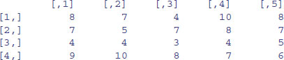
Thus, the four random numbers in the first trial were 8, 7, 4 and 9 (i.e. column 1). To learn more about sapply, see p. 63.
2.10 Loops and repeats
The classic, Fortran-like loop is available in R. The syntax is a little different, but the idea is identical; you request that an index, i, takes on a sequence of values, and that one or more lines of commands are executed as many times as there are different values of i. Here is a loop executed five times with the values of i from 1 to 5; we print the square of each value:
for (i in 1:5) print(i^2)
[1] 1
[1] 4
[1] 9
[1] 16
[1] 25
For multiple lines of code, you use curly brackets {} to enclose material over which the loop is to work. Note that the ‘hard return’ (the Enter key) at the end of each command line is an essential part of the structure (you can replace the hard returns by semicolons if you like, but clarity is improved if you put each command on a separate line):
j <- k <- 0
for (i in 1:5) {
j <- j+1
k <- k+i*j
print(i+j+k) }
[1] 3
[1] 9
[1] 20
[1] 38
[1] 65
Here we use a for loop to write a function to calculate factorial x (written x!) which is

So 4! = 4 × 3 × 2 = 24. Here is the function:
fac1 <- function(x) {
f <- 1
if (x<2) return (1)
for (i in 2:x) {
f <- f*i}
f }
That seems rather complicated for such a simple task, but we can try it out for the numbers 0 to 5:
sapply(0:5,fac1)
[1] 1 1 2 6 24 120
There are two other looping functions in R: repeat and while. We demonstrate their use for the purpose of illustration, but we can do much better in terms of writing a compact function for finding factorials (see below). First, the while function:
fac2 <- function(x) {
f <- 1
t <- x
while(t>1) {
f <- f*t
t <- t-1 }
return(f) }
The key point is that if you want to use while, you need to set up an indicator variable (t in this case) and change its value within each iteration (t <- t-1). We test the function on the numbers 0 to 5:
sapply(0:5,fac2)
[1] 1 1 2 6 24 120
Finally, we demonstrate the use of the repeat function:
fac3 <- function(x) {
f <- 1
t <- x
repeat {
if (t<2) break
f <- f*t
t <- t-1 }
return(f) }
Because the repeat function contains no explicit limit, you need to be careful not to program an infinite loop. You must include a logical escape clause that leads to a break command:
sapply(0:5,fac3)
[1] 1 1 2 6 24 120
It is almost always better to use a built-in function that operates on the entire vector and hence removes the need for loops or repeats of any sort. In this case, we can make use of the cumulative product function, cumprod. Here it is in action:
cumprod(1:5)
[1] 1 2 6 24 120
This is already pretty close to what we need for our factorial function. It does not work for 0! of course, because the whole vector would end up full of zeros if the first element in the vector was zero (try 0:5 and see). The factorial of x > 0 is the maximum value from the vector produced by cumprod:
fac4 <- function(x) max(cumprod(1:x))
This definition has the desirable side effect that it also gets 0! correct, because when x is 0 the function finds the maximum of 1 and 0 which is 1.
max(cumprod(1:0))
[1] 1
sapply(0:5,fac4)
[1] 1 1 2 6 24 120
Alternatively, you could adapt an existing built-in function to do the job. x! is the same as Γ(x + 1), so
fac5 <- function(x) gamma(x+1)
sapply(0:5,fac5)
[1] 1 1 2 6 24 120
Until quite recently there was no built-in factorial function in R, but now there is:
sapply(0:5,factorial)
[1] 1 1 2 6 24 120
2.10.1 Creating the binary representation of a number
Here is a function that uses the while function in converting a specified number to its binary representation. The trick is that the smallest digit (0 for even or 1 for odd numbers) is always at the right-hand side of the answer (in location 32 in this case):
binary <- function(x) {
i <- 0
string <- numeric(32)
while(x>0) {
string[32-i]< -x %% 2
x <- x%% 2
i <- i+1 }
first <- match(1,string)
string[first:32] }
The leading zeros (1 to first – 1) within the string are not printed. We run the function to find the binary representation of the numbers 15 to 17:
sapply(15:17,binary)
[[1]]
[1] 1 1 1 1
[[2]]
[1] 1 0 0 0 0
[[3]]
[1] 1 0 0 0 1
The next function uses while to generate the Fibonacci series 1, 1, 2, 3, 5, 8, … in which each term is the sum of its two predecessors. The key point about while loops is that the logical variable controlling their operation is altered inside the loop. In this example, we alter n, the number whose Fibonacci number we want, starting at n, reducing the value of n by 1 each time around the loop, and ending when n gets down to 0. Here is the code:
fibonacci <- function(n) {
a <- 1
b <- 0
while(n>0)
{swap <- a
a <- a+b
b <- swap
n <- n-1 }
b }
An important general point about computing involves the use of the swap variable above. When we replace a by a + b on line 6 we lose the original value of a. If we had not stored this value in swap, we could not set the new value of b to the old value of a on line 7. Now test the function by generating the Fibonacci numbers 1 to 10:
sapply(1:10,fibonacci)
[1] 1 1 2 3 5 8 13 21 34 55
2.10.2 Loop avoidance
It is good R programming practice to avoid using loops wherever possible. The use of vector functions (p. 41) makes this particularly straightforward in many cases. Suppose that you wanted to replace all of the negative values in an array by zeros. In the old days, you might have written something like this:
for (i in 1:length(y)) { if(y[i] < 0) y[i] <- 0 }
Now, however, you would use logical subscripts (p. 39) like this:
y[y<0] <- 0
The ifelse function
Sometimes you want to do one thing if a condition is true and a different thing if the condition is false (rather than do nothing, as in the last example). The ifelse function allows you to do this for entire vectors without using for loops. We might want to replace any negative values of y by –1 and any positive values and zero by +1:
z <- ifelse (y < 0, -1, 1)
Next we use ifelse to convert the continuous variable called Area into a new, two-level factor with values big and small defined by the median Area of the fields:
data <- read.table("c:\\temp\\worms.txt",header=T)
attach(data)
ifelse(Area>median(Area),"big","small")

You should use the much more powerful function called cut when you want to convert a continuous variable like Area into many levels (p. 838).
Another use of ifelse is to override R's natural inclinations. The log of zero in R is -Inf, as you see in these 20 random numbers from a Poisson process with a mean count of 1.5:
y <- log(rpois(20,1.5))
y
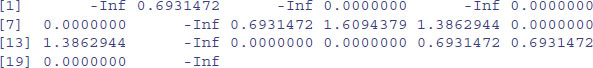
However, if we want the log of zero to be represented by NA in our particular application we can write:
ifelse(y<0,NA,y)
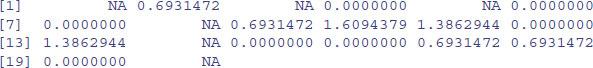
2.10.3 The slowness of loops
To see how slow loops can be, we compare two ways of finding the maximum number in a vector of 10 million random numbers from a uniform distribution:
x <- runif(10000000)
First, using the vector function max:
system.time(max(x))
user system elapsed
0.03 0.00 0.03
As you see, this operation took just 0.03 seconds to solve using the vector function max to look at the 10 million numbers in x. Using a loop, however, took more than 9 seconds:
pc <- proc.time()
cmax <- x[1]
for (i in 2:10000000) {
if(x[i]>cmax) cmax <- x[i] }
proc.time()-pc
user system elapsed
9.39 0.13 9.51
The functions system.time and proc.time produce a vector of three numbers, showing the user, system and total elapsed times for the currently running R process. It is the third number (elapsed time in seconds, 9.51 in this case) that is typically the most useful.
2.10.4 Do not ‘grow’ data sets by concatenation or recursive function calls
Here is an extreme example of what not to do. We want to create a vector containing 100 000 numbers in sequence from 1 to 100 000. First, the quickest way using the built-in sequence generator which is invoked by the colon symbol (:)
test1 <- function(){
y <- 1:100000
}
Now we obtain the same result using a loop, where we tell R in advance how long the final vector is going to be, using the numeric function. This is called preallocation.
test2 <- function(){
y <- numeric(100000)
for (i in 1:100000) y[i] <- i
}
Finally, the most inefficient way. Each time we go round the loop we concatenate the new value onto the right-hand end of the vector that has been created up to this point. We start with a NULL vector, then build it up, one step at a time, which looks like a neat idea, but is extremely inefficient, because changing the size of a vector takes roughly the same size as setting a vector up from scratch, and we change the length of our vector 100 000 times in this example. This ill-advised procedure is called re-dimensioning.
test3 <- function(){
y <- NULL
for (i in 1:100000) y <- c(y,i)
}
To compare the efficiency of the three methods, we shall work out how long each takes to complete the task. The function called proc.time determines how much real time and computer processing unit (CPU) time (in seconds) the currently running R process has already taken:
proc.time()
user system elapsed
53.15 5.14 2483.00
The user time is the CPU time charged for the execution of user instructions of the calling process, the system time is the CPU time charged for execution by the system on behalf of the calling process, and the elapsed time includes other stuff that the computer is doing, unrelated to your R session.
The function system.time calls the function proc.time, then evaluates your expression, and then calls proc.time once more, returning the difference between the two proc.time calls as its output. We can compare the efficiencies of our three different functions using system.time like this:
system.time(test1())
user system elapsed
0 0 0
system.time(test2())
user system elapsed
0.16 0.02 0.17
system.time(test3())
user system elapsed
8.95 0.02 8.97
The first method is so lightening fast that it does not even register on the clock. The loop using a pre-determined vector length is also very fast (0.16 seconds). In contrast, the last method, where we grew the vector at each iteration, is staggeringly slow (8.95 seconds). The moral: do not grow vectors by repeated concatenation.
2.10.5 Loops for producing time series
Wherever we can, we use vectorized functions in R because this leads to compact, efficient and easily readable code. Sometimes, however, we need to resort to using loops. Suppose we are interested in the dynamics of a population which is governed by two parameters: the per capita reproductive rate (λ) and the maximum supportable population (Nmax), which for convenience we shall set to 1.0). Next year's population N(t+1) is given by this year's population, N(t), multiplied by lambda, multiplied again by the fraction of Nmax that is currently unrealized (i.e. (Nmax - N(t))/Nmax = 1 - N(t) in the current case). Thus, we have a difference equation

To simulate the dynamics of this population in R, we start by writing the difference equation as a function (call it next.year for instance):
next.year <- function(x) lambda * x * (1 - x)
So if we begin with a population of N = 0.6 and set λ = 3.7 we can predict next year's population like this:
lambda <- 3.7
next.year(0.6)
[1] 0.888
The population has increased by 48% (0.888 / 0.6 = 1.48). What happens in the second year?
next.year(0.888)
[1] 0.3679872
The population crashes to less than half its previous value (0.367 987 2/0.888 = 0.4144). We could go on repeating these calculations, modelling year after year, but this is an obvious case where using a loop would be the best solution. Let us assume that we want to model the population over 20 years. It is good practice in cases like this to define a vector to contain the 20 population sizes at the outset (preallocation) using numeric like this:
N <- numeric(20)
We set the initial population size (0.6) like this:
N[1] <- 0.6
Now if we run through a loop to simulate the years 2 through 20 using an index called t (for time), we can invoke the function called next.year repeatedly, employing t as a subscript like this:
for (t in 2:20) N[t] <- next.year(N[t-1])
Finally, we might want to plot a time series of the population dynamics over the course of 20 years.
plot(N,type="l")
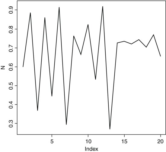
This famous difference equation is known as the quadratic map, and it played a central role in the development of chaos theory (May, 1974). For large values of λ (as we used in the example above), the function is capable of producing series of numbers that are, to all intents and purposes, random. This led to a definition of chaos as behaviour that exhibited extreme sensitivity to initial conditions: tiny differences in initial population size would lead to radically different time series in population dynamics.