2.11 Lists
Lists are extremely important objects in R. You will have heard of the problems of ‘comparing apples and oranges’ or how two things are ‘as different as chalk and cheese’. You can think of lists as a way of getting around these problems. Here are four completely different objects: a numeric vector, a logical vector, a vector of character strings and a vector of complex numbers:
apples <- c(4,4.5,4.2,5.1,3.9)
oranges <- c(TRUE, TRUE, FALSE)
chalk <- c("limestone", "marl","oolite", "CaC03")
cheese <- c(3.2-4.5i,12.8+2.2i)
We cannot bundle them together into a dataframe, because the vectors are of different lengths:
data.frame(apples,oranges,chalk,cheese)
Error in data.frame(apples, oranges, chalk, cheese) :
arguments imply differing number of rows: 5, 3, 4, 2
Despite their differences, however, we can bundle them together in a single list called items:
items <- list(apples,oranges,chalk,cheese)
items
[[1]]
[1] 4.0 4.5 4.2 5.1 3.9
[[2]]
[1] TRUE TRUE FALSE
[[3]]
[1] "limestone" "marl" "oolite" "CaC03"
[[4]]
[1] 3.2-4.5i 12.8+2.2i
Subscripts on vectors, matrices, arrays and dataframes have one set of square brackets [6], [3,4] or [2,3,2,1], but subscripts on lists have double square brackets [[2]] or [[i,j]]. If we want to extract the chalk from the list, we use subscript [[3]]:
items[[3]]
[1] "limestone" "marl" "oolite" "CaC03"
If we want to extract the third element within chalk (oolite) then we use single subscripts after the double subscripts like this:
items[[3]][3]
[1] "oolite"
R is forgiving about failure to use double brackets on their own, but not when you try to access a component of an object within a list:
items[3]
[[1]]
[1] "limestone" "marl" "oolite" "CaC03"
items[3][3]
[[1]]
NULL
There is another indexing convention in R which is used to extract named components from lists using the element names operator $. This is known as ‘indexing tagged lists’. For this to work, the elements of the list must have names. At the moment our list called items has no names:
names(items)
NULL
You can give names to the elements of a list in the function that creates the list by using the equals sign like this:
items <- list(first=apples,second=oranges,third=chalk,fourth=cheese)
Now you can extract elements of the list by name
items$fourth
[1] 3.2-4.5i 12.8+2.2i
2.11.1 Lists and lapply
We can ask a variety of questions about our new list object:
class(items)
[1] "list"
mode(items)
[1] "list"
is.numeric(items)
[1] FALSE
is.list(items)
[1] TRUE
length(items)
[1] 4
Note that the length of a list is the number of items in the list, not the lengths of the individual vectors within the list.
The function lapply applies a specified function to each of the elements of a list in turn (without the need for specifying a loop, and not requiring us to know how many elements there are in the list). A useful function to apply to lists is the length function; this asks how many elements comprise each component of the list. Technically we want to know the length of each of the vectors making up the list:
lapply(items,length)
$first
[1] 5
$second
[1] 3
$third
[1] 4
$fourth
[1] 2
This shows that items consists of four vectors, and shows that there were 5 elements in the first vector, 3 in the second 4 in the third and 2 in the fourth. But 5 of what, and 3 of what? To find out, we apply the function class to the list:
lapply(items,class)
$first
[1] "numeric"
$second
[1] "logical"
$third
[1] "character"
$fourth
[1] "complex"
So the answer is there were 5 numbers in the first vector, 3 logical variables in the second, 4 character strings in the third vector and 2 complex numbers in the fourth.
Applying numeric functions to lists will only work for objects of class numeric or complex, or objects (like logical values) that can be coerced into numbers. Here is what happens when we use lapply to apply the function mean to items:
lapply(items,mean)
$first
[1] 4.34
$second
[1] 0.6666667
$third
[1] NA
$fourth
[1] 8-1.15i
Warning message:
In mean.default(X[[3L]], …) :
argument is not numeric or logical: returning NA
We get a warning message pointing out that the third vector cannot be coerced to a number (it is not numeric, complex or logical), so NA appears in the output. The second vector produces the answer 2/3 because logical false (FALSE) is coerced to numeric 0 and logical true (TRUE) is coerced to numeric 1.
The summary function works for lists:
summary(items)
Length Class Mode
first 5 -none- numeric
second 3 -none- logical
third 4 -none- character
fourth 2 -none- complex
but the most useful overview of the contents of a list is obtained with str, the structure function:
str(items)
List of 4
$ first : num [1:5] 4 4.5 4.2 5.1 3.9
$ second: logi [1:3] TRUE TRUE FALSE
$ third : chr [1:4] "limestone" "marl" "oolite" "CaC03"
$ fourth: cplx [1:2] 3.2-4.5i 12.8+2.2i
2.11.2 Manipulating and saving lists
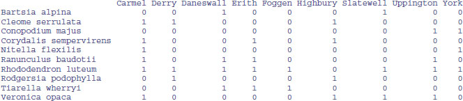
Saving lists to files is tricky, because lists typically have different numbers of items in each row so we cannot use write.table. Here is a dataframe on species presence (1) or absence (0), with species' Latin binomials in the first column as the row names:
data<-read.csv("c:\\temp\\pa.csv",row.names=1)
data
There are two kinds of operations you might want to do with a dataframe like this:
- produce lists of the sites at which each species is found;
- produce lists of the species found in any given site.
We shall do each of these tasks in turn.
The issue is that the numbers of place names differ from species to species, and the numbers of species differ from place to place. However, it is easy to create a list showing the column numbers that contain locations for each species:
sapply(1:10,function(i) which(data[i,]>0))
[[1]]
[1] 3 7
[[2]]
[1] 1 2 6
[[3]]
[1] 8 9
[[4]]
[1] 1 4 6
[[5]]
[1] 1 9
[[6]]
[1] 1 3 4 8
[[7]]
[1] 1 2 3 4 5 7 8 9
[[8]]
[1] 2 6
[[9]]
[1] 3 4 5
[[10]]
[1] 1 6 7 8
This indicates that Bartsia alpina (the first species) is found in locations 3 and 7 (Daneswall and Slatewell). If we save this list (calling it spp for instance), then we can extract the column names at which each species is present, using the elements of spp as subscripts on the column names of data, like this:
spp<-sapply(1:10,function(i) which(data[i,]>0))
sapply(1:10, function(i)names(data)[spp[[i]]] )
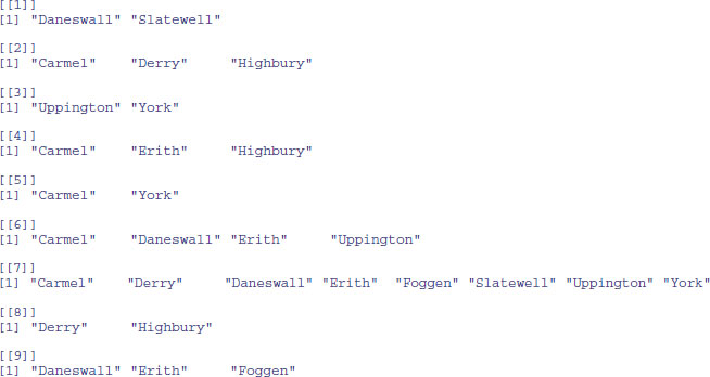

This completes the first task.
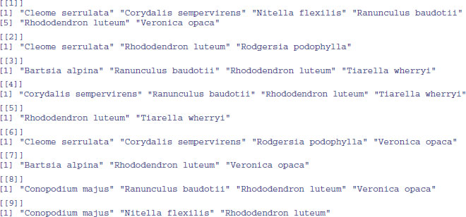
The second task is to get species lists for each location. We apply a similar method to extract the appropriate species (this time from rownames(data)) on the basis that the presence score for this site is data[,j] > 0:
sapply(1:9, function (j) rownames(data)[data[,j]>0] )
Because the species lists for different sites are of different lengths, the simplest solution is to create a separate file for each species list. We need to create a set of nine file names incorporating the site name, then use write.table in a loop:
spplists<-sapply(1:9, function (j) rownames(data)[data[,j]>0] )
for (i in 1:9) {
slist<-data.frame(spplists[[i]])
names(slist)<-names(data)[i]
fn<-paste("c:\\temp\\",names(data)[i],".txt",sep="")
write.table(slist,fn)
}
We have produced nine separate files. Here, for instance, are the contents of the file called c:\\temp\\Carmel.txt as viewed in a text editor like Notepad:
"Carmel"
"1" "Cleome serrulata"
"2" "Corydalis sempervirens"
"3" "Nitella flexilis"
"4" "Ranunculus baudotii"
"5" "Rhododendron luteum"
"6" "Veronica opaca"
Perhaps the simplest and best solution is to turn the whole presence/absence matrix into a dataframe. Then both tasks become very straightforward. Start by using stack to create a dataframe of place names and presence/absence information:
newframe<-stack(data)
head(newframe)
values ind
1 0 Carmel
2 1 Carmel
3 0 Carmel
4 1 Carmel
5 1 Carmel
6 1 Carmel
Now extract the species names from the row names, repeat the list of names nine times, and add the resulting vector species names to the dataframe:
newframe<-data.frame(newframe, rep(rownames(data),9))
Finally, give the three columns of the new dataframe sensible names:
names(newframe)<-c("present","location","species")
head(newframe)
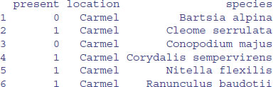
Unlike the lists, you can easily save this object to file:
write.table(newframe,"c:\\temp\\spplists.txt")
Now it is simple to do both our tasks. Here a location list for species = Bartsia alpina:
newframe[newframe$species=="Bartsia alpina" & newframe$present==1,2]
[1] Daneswall Slatewell
and here is a species list for location = Carmel:
newframe[newframe$location=="Carmel" & newframe$present==1,3]

Lists are great, but dataframes are better. The cost of the dataframe is the potentially substantial redundancy in storage requirement. In practice, with relatively small dataframes, this seldom matters.
2.12 Text, character strings and pattern matching
In R, character strings are defined by double quotation marks:
a <- "abc"
b <- "123"
Numbers can be coerced to characters (as in b above), but non-numeric characters cannot be coerced to numbers:
as.numeric(a)
[1] NA
Warning message:
NAs introduced by coercion
as.numeric(b)
[1] 123
One of the initially confusing things about character strings is the distinction between the length of a character object (a vector), and the numbers of characters (nchar) in the strings that comprise that object. An example should make the distinction clear:
pets <- c("cat","dog","gerbil","terrapin")
Here, pets is a vector comprising four character strings:
length(pets)
[1] 4
and the individual character strings have 3, 3, 6 and 7 characters, respectively:
nchar(pets)
[1] 3 3 6 7
When first defined, character strings are not factors:
class(pets)
[1] "character"
is.factor(pets)
[1] FALSE
However, if the vector of characters called pets was part of a dataframe (e.g. if it was input using read.table) then R would coerce all the character variables to act as factors:
df <- data.frame(pets)
is.factor(df$pets)
[1] TRUE
There are built-in vectors in R that contain the 26 letters of the alphabet in lower case (letters) and in upper case (LETTERS):
letters
[1] "a" "b" "c" "d" "e" "f" "g" "h" "i" "j" "k" "l" "m" "n" "o" "p"
[17] "q" "r" "s" "t" "u" "v" "w" "x" "y" "z"
LETTERS
[1] "A" "B" "C" "D" "E" "F" "G" "H" "I" "J" "K" "L" "M" "N" "O" "P"
[17] "Q" "R" "S" "T" "U" "V" "W" "X" "Y" "Z"
To discover which number in the alphabet the letter n is, you can use the which function like this:
which(letters=="n")
[1] 14
For the purposes of printing you might want to suppress the quotes that appear around character strings by default. The function to do this is called noquote:
noquote(letters)
[1] a b c d e f g h i j k l m n o p q r s t u v w x y z
2.12.1 Pasting character strings together
You can amalgamate individual strings into vectors of character information:
c(a,b)
[1] "abc" "123"
This shows that the concatenation produces a vector of two strings. It does not convert two 3-character strings into one 6-character string. The R function to do that is paste:
paste(a,b,sep="")
[1] "abc123"
The third argument, sep="", means that the two character strings are to be pasted together without any separator between them: the default for paste is to insert a single blank space, like this:
paste(a,b)
[1] "abc 123"
Notice that you do not lose blanks that are within character strings when you use the sep="" option in paste.
paste(a,b," a longer phrase containing blanks",sep="")
[1] "abc123 a longer phrase containing blanks"
If one of the arguments to paste is a vector, each of the elements of the vector is pasted to the specified character string to produce an object of the same length as the vector:
d <- c(a,b,"new")
e <- paste(d,"a longer phrase containing blanks")
e
[1] "abc a longer phrase containing blanks"
[2] "123 a longer phrase containing blanks"
[3] "new a longer phrase containing blanks"
You may need to think about why there are three lines of output.
In this next example, we have four fields of information and we want to paste them together to make a file path for reading data into R:
drive <- "c:"
folder <- "temp"
file <- "file"
extension <- ".txt"
Now use the function paste to put them together:
paste(drive, folder, file, extension)
[1] "c: temp file .txt"
This has the essence of what we want, but it is not quite there yet. We need to replace the blank spaces " " that are the default separator with "" no space, and to insert slashes "\\" between the drive and the directory, and the directory and file names:
paste(drive, "\\",folder, "\\",file, extension,sep="")
[1] "c:\\temp\\file.txt"
2.12.2 Extracting parts of strings
We being by defining a phrase:
phrase <- "the quick brown fox jumps over the lazy dog"
The function called substr is used to extract substrings of a specified number of characters from within a character string. Here is the code to extract the first, the first and second, the first, second and third,…, the first 20 characters from our phrase:
q <- character(20)
for (i in 1:20) q[i] <- substr(phrase,1,i)
q

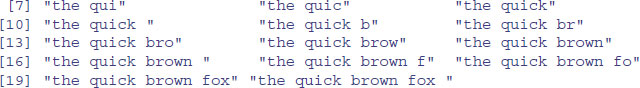
The second argument in substr is the number of the character at which extraction is to begin (in this case always the first), and the third argument is the number of the character at which extraction is to end (in this case, the ith).
2.12.3 Counting things within strings
Counting the total number of characters in a string could not be simpler; just use the nchar function directly, like this:
nchar(phrase)
[1] 43
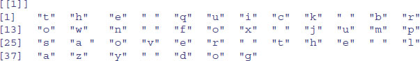
So there are 43 characters including the blanks between the words. To count the numbers of separate individual characters (including blanks) you need to split up the character string into individual characters (43 of them), using strsplit like this:
strsplit(phrase,split=character(0))
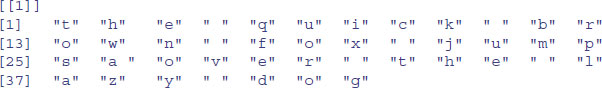
You could use NULL in place of split=character(0) (see below). The table function can then be used for counting the number of occurrences of each of the characters:
table(strsplit(phrase,split=character(0)))
a b c d e f g h i j k l m n o p q r s t u v w x y z
8 1 1 1 1 3 1 1 2 1 1 1 1 1 1 4 1 1 2 1 2 2 1 1 1 1 1
This demonstrates that all of the letters of the alphabet were used at least once within our phrase, and that there were eight blanks within the string called phrase. This suggests a way of counting the number of words in a phrase, given that this will always be one more than the number of blanks (so long as there are no leading or trailing blanks in the string):
words <- 1+table(strsplit(phrase,split=character(0)))[1]
words
9
What about the lengths of the words within phrase? Here are the separate words:
strsplit(phrase, " ")
[[1]]
[1] "the" "quick" "brown" "fox" "jumps" "over" "the" "lazy" "dog"
We work out their lengths using lapply to apply the function nchar to each element of the list produced by strsplit. Then we use table to count how many words of each length are present:
table(lapply(strsplit(phrase, " "), nchar))
3 4 5
4 2 3
showing there were 4 three-letter words, 2 four-letter words and 3 five-letter words.
This is how you reverse a character string. The logic is that you need to break it up into individual characters, then reverse their order, then paste them all back together again. It seems long-winded until you think about what the alternative would be:
strsplit(phrase,NULL)
lapply(strsplit(phrase,NULL),rev)
[[1]]

sapply(lapply(strsplit(phrase, NULL), rev), paste, collapse="")
[1] "god yzal eht revo spmuj xof nworb kciuq eht"
The collapse argument is necessary to reduce the answer back to a single character string. Note that the word lengths are retained, so this would be a poor method of encryption.
When we specify a particular string to form the basis of the split, we end up with a list made up from the components of the string that do not contain the specified string. This is hard to understand without an example. Suppose we split our phrase using ‘the’:
strsplit(phrase,"the")
[[1]]
[1] "" " quick brown fox jumps over " " lazy dog"
There are three elements in this list: the first one is the empty string "" because the first three characters within phrase were exactly ‘the’; the second element contains the part of the phrase between the two occurrences of the string ‘the’; and the third element is the end of the phrase, following the second ‘the’. Suppose that we want to extract the characters between the first and second occurrences of ‘the’. This is achieved very simply, using subscripts to extract the second element of the list:
strsplit(phrase,"the")[[1]] [2]
[1] " quick brown fox jumps over "
Note that the first subscript in double square brackets refers to the number within the list (there is only one list in this case), and the second subscript refers to the second element within this list. So if we want to know how many characters there are between the first and second occurrences of the word ‘the’ within our phrase, we put:
nchar(strsplit(phrase,"the")[[1]] [2])
[1] 28
2.12.4 Upper- and lower-case text
It is easy to switch between upper and lower cases using the toupper and tolower functions:
toupper(phrase)
[1] THE QUICK BROWN FOX JUMPS OVER THE LAZY DOG"
tolower(toupper(phrase))
[1] "the quick brown fox jumps over the lazy dog"
2.12.5 The match function and relational databases
The match function answers the question: ‘Where (if at all) do the values in the second vector appear in the first vector?’ It is a really important function, but it is impossible to understand without an example:
first <- c(5,8,3,5,3,6,4,4,2,8,8,8,4,4,6)
second <- c(8,6,4,2)
match(first,second)
[1] NA 1 NA NA NA 2 3 3 4 1 1 1 3 3 2
The first thing to note is that match produces a vector of subscripts (index values) and that these are subscripts within the second vector. The length of the vector produced by match is the length of the first vector (15 in this example). If elements of the first vector do not occur anywhere in the second vector, then match produces NA. It works like this. Where does 5 (from the first position in the first vector) appear in the second vector? Answer: it does not (NA). Then, where does 8 (the second element of the first vector) appear in the second vector? Answer: in position number 1. And so on. Why would you ever want to use this? The answer turns out to be very general and extremely useful in data management.
Large and/or complicated databases are always best stored as relational databases (e.g. Oracle or Access). In these, data are stored in sets of two-dimensional spreadsheet-like objects called tables. Data are divided into small tables with strict rules as to what data they can contain. You then create relationships between the tables that allow the computer to look from one table to another in order to assemble the data you want for a particular application. The relationship between two tables is based on fields whose values (if not their variable names) are common to both tables. The rules for constructing effective relational databases were first proposed by Dr E.F. Codd of the IBM Research Laboratory at San Jose, California, in an extremely influential paper in 1970:
- All data are in tables.
- There is a separate table for each set of related variables.
- The order of the records within tables is irrelevant (so you can add records without reordering the existing records).
- The first column of each table is a unique ID number for every row in that table (a simple way to make sure that this works is to have the rows numbered sequentially from 1 at the top, so that when you add new rows you are sure that they get unique identifiers).
- There is no unnecessary repetition of data so the storage requirement is minimized, and when we need to edit a record, we only need to edit it once (the last point is very important).
- Each piece of data is ‘granular’ (meaning as small as possible); so you would split a customer's name into title (Dr), first name (Charles), middle name (Urban), surname (Forrester), and preferred form of address (Chuck), so that if they were promoted, for instance, we would only need to convert Dr to Prof. in the title field.
These are called the ‘normalization rules’ for creating bullet-proof databases. The use of Structured Query Language (SQL) in R to interrogate relational databases is discussed in Chapter 3 (p. 154). Here, the only point is to see how the match function relates information in one vector (or table) to information in another.
Take a medical example. You have a vector containing the anonymous identifiers of nine patients (subjects):
subjects <- c("A", "B", "G", "M", "N", "S", "T", "V", "Z")
Suppose you wanted to give a new drug to all the patients identified in the second vector called suitable.patients, and the conventional drug to all the others. Here are the suitable patients:
suitable.patients <- c("E", "G", "S", "U", "Z")
Notice that there are several suitable patients who are not part of this trial (E and U). This is what the match function does:
match(subjects, suitable.patients)
[1] NA NA 2 NA NA 3 NA NA 5
For each of the individuals in the first vector (subjects) it finds the subscript in the second vector (suitable patients), returning NA if that patient does not appear in the second vector. The key point to understand is that the vector produced by match is the same length as the first vector supplied to match, and that the numbers in the result are subscripts within the second vector. The last bit is what people find hard to understand at first.
Let us go through the output term by term and see what each means. Patient A is not in the suitable vector, so NA is returned. The same is true for patient B. Patient G is suitable, so we get a number in the third position. That number is a 2 because patient G is the second element of the vector called suitable.patients. Neither patient M nor N is in the second vector, so they both appear as NA. Patient S is suitable and so produces a number. The number is 3 because that is the position of S with the second vector.
To complete the job, we want to produce a vector of the drugs to be administered to each of the subjects. We create a vector containing the two treatment names:
drug <- c("new", "conventional")
Then we use the result of the match to give the right drug to the right patient:
drug[ifelse(is.na(match(subjects, suitable.patients)),2,1)]
[1] "conventional" "conventional" "new" "conventional"
[5] "conventional" "new" "conventional" "conventional"
[9] "new"
Note the use of ifelse with is.na to produce a subscript 2 (to use with drug) for the unsuitable patients, and a 1 when the result of the match is not NA (i.e. for the suitable patients). You may need to work through this example several times (but it is well worth mastering it).
2.12.6 Pattern matching
We need a dataframe with a serious amount of text in it to make these exercises relevant:
wf <- read.table("c:\\temp\\worldfloras.txt",header=T)
attach(wf)
names(wf)
[1] "Country" "Latitude" "Area" "Population" "Flora"
[6] "Endemism" "Continent"
Country
As you can see, there are 161 countries in this dataframe (strictly, 161 places, since some of the entries, such as Sicily and Balearic Islands, are not countries). The idea is that we want to be able to select subsets of countries on the basis of specified patterns within the character strings that make up the country names (factor levels). The function to do this is grep. This searches for matches to a pattern (specified in its first argument) within the character vector which forms the second argument. It returns a vector of indices (subscripts) within the vector appearing as the second argument, where the pattern was found in whole or in part. The topic of pattern matching is very easy to master once the penny drops, but it hard to grasp without simple, concrete examples. Perhaps the simplest task is to select all the countries containing a particular letter – for instance, upper-case R:
as.vector(Country[grep("R",as.character(Country))])
[1] "Central African Republic" "Costa Rica"
[3] "Dominican Republic" "Puerto Rico"
[5] "Reunion" "Romania"
[7] "Rwanda" "USSR"
To restrict the search to countries whose first name begins with R use the ^ character like this:
as.vector(Country[grep("^ R",as.character(Country))])
[1] "Reunion" "Romania" "Rwanda"
To select those countries with multiple names with upper-case R as the first letter of their second or subsequent names, we specify the character string as “blank R” like this:
as.vector(Country[grep(" R",as.character(Country)])
[1] "Central African Republic" "Costa Rica"
[3] "Dominican Republic" "Puerto Rico"
To find all the countries with two or more names, just search for a blank " ":
as.vector(Country[grep(" ",as.character(Country))])
[1] "Balearic Islands" "Burkina Faso"
[3] "Central African Republic" "Costa Rica"
[5] "Dominican Republic" "El Salvador"
[7] "French Guiana" "Germany East"
[9] "Germany West" "Hong Kong"
[11] "Ivory Coast" "New Caledonia"
[13] "New Zealand" "Papua New Guinea"
[15] "Puerto Rico" "Saudi Arabia"
[17] "Sierra Leone" "Solomon Islands"
[19] "South Africa" "Sri Lanka"
[21] "Trinidad & Tobago" "Tristan da Cunha"
[23] "United Kingdom" "Viet Nam"
[25] "Yemen North" "Yemen South"
To find countries with names ending in ‘y’ use the $ symbol like this:
as.vector(Country[grep("y$",as.character(Country))])
[1] "Hungary" "Italy" "Norway" "Paraguay" "Sicily" "Turkey"
[7] "Uruguay"
To recap: the start of the character string is denoted by ^ and the end of the character string is denoted by $. For conditions that can be expressed as groups (say, series of numbers or alphabetically grouped lists of letters), use square brackets inside the quotes to indicate the range of values that is to be selected. For instance, to select countries with names containing upper-case letters from C to E inclusive, write:
as.vector(Country[grep("[C-E]",as.character(Country))])
[1] "Cameroon" "Canada"
[3] "Central African Republic" "Chad"
[5] "Chile" "China"
[7] "Colombia" "Congo"
[9] "Corsica" "Costa Rica"
[11] "Crete" "Cuba"
[13] "Cyprus" "Czechoslovakia"
[15] "Denmark" "Dominican Republic"
[17] "Ecuador" "Egypt"
[19] "El Salvador" "Ethiopia"
[21] "Germany East" "Ivory Coast"
[23] "New Caledonia" "Tristan da Cunha"
Notice that this formulation picks out countries like Ivory Coast and Tristan da Cunha that contain upper-case Cs in places other than as their first letters. To restrict the choice to first letters use the ^ operator before the list of capital letters:
as.vector(Country[grep("^[C-E]",as.character(Country))])
[1] "Cameroon" "Canada"
[3] "Central African Republic" "Chad"
[5] "Chile" "China"
[7] "Colombia" "Congo"
[9] "Corsica" "Costa Rica"
[11] "Crete" "Cuba"
[13] "Cyprus" "Czechoslovakia"
[15] "Denmark" "Dominican Republic"
[17] "Ecuador" "Egypt"
[19] "El Salvador" "Ethiopia"
How about selecting the counties not ending with a specified patterns? The answer is simply to use negative subscripts to drop the selected items from the vector. Here are the countries that do not end with a letter between ‘a’ and ‘t’:
as.vector(Country[-grep("[a-t]$",as.character(Country))])
[1] "Hungary" "Italy" "Norway" "Paraguay" "Peru" "Sicily"
[7] "Turkey" "Uruguay" "USA" "USSR" "Vanuatu"
You see that USA and USSR are included in the list because we specified lower-case letters as the endings to omit. To omit these other countries, put ranges for both upper- and lower-case letters inside the square brackets, separated by a space:
as.vector(Country[-grep("[A-T a-t]$",as.character(Country))])
[1] "Hungary" "Italy" "Norway" "Paraguay" "Peru" "Sicily"
[7] "Turkey" "Uruguay" "Vanuatu"
2.12.7 Dot . as the ‘anything’ character
Countries with ‘y’ as their second letter are specified by ^.y. The ^ shows ‘starting’, then a single dot means one character of any kind, so y is the specified second character:
as.vector(Country[grep("^.y",as.character(Country))])
[1] "Cyprus" "Syria"
To search for countries with ‘y’ as third letter:
as.vector(Country[grep("^..y",as.character(Country))])
[1] "Egypt" "Guyana" "Seychelles"
If we want countries with ‘y’ as their sixth letter:
as.vector(Country[grep("^.{5}y",as.character(Country))])
[1] "Norway" "Sicily" "Turkey"
(Five ‘anythings’ is shown by ‘.’ then curly brackets {5} then y.) Which are the countries with four or fewer letters in their names?
as.vector(Country[grep("^.{,4}$",as.character(Country))])
[1] "Chad" "Cuba" "Iran" "Iraq" "Laos" "Mali" "Oman"
[8] "Peru" "Togo" "USA" "USSR"
The ‘.’ means ‘anything’ while the {,4} means ‘repeat up to four’ anythings (dots) before $ (the end of the string). So to find all the countries with 15 or more characters in their name:
as.vector(Country[grep("^.{15,}$",as.character(Country))])
[1] "Balearic Islands" "Central African Republic"
[3] "Dominican Republic" "Papua New Guinea"
[5] "Solomon Islands" "Trinidad & Tobago"
[7] "Tristan da Cunha"
2.12.8 Substituting text within character strings
Search-and-replace operations are carried out in R using the functions sub and gsub. The two substitution functions differ only in that sub replaces only the first occurrence of a pattern within a character string, whereas gsub replaces all occurrences. An example should make this clear. Here is a vector comprising seven character strings, called text:
text <- c("arm", "leg", "head", "foot", "hand", "hindleg" "elbow")
We want to replace all lower-case ‘h’ with upper-case ‘H’:
gsub("h","H",text)
[1] "arm" "leg" "Head" "foot" "Hand" "Hindleg" "elbow"
Now suppose we want to convert the first occurrence of a lower-case ‘o’ into an upper-case ‘O’. We use sub for this (not gsub):
sub("o","O",text)
[1] "arm" "leg" "head" "fOot" "hand" "hindleg" "elbOw"
You can see the difference between sub and gsub in the following, where both instances of ‘o’ in foot are converted to upper case by gsub but not by sub:
gsub("o","O",text)
[1] "arm" "leg" "head" "fOOt" "hand" "hindleg" "elbOw"
More general patterns can be specified in the same way as we learned for grep (above). For instance, to replace the first character of every string with upper-case ‘O’ we use the dot notation (. stands for ‘anything’) coupled with ^ (the ‘start of string’ marker):
gsub("^.","O",text)
[1] "Orm" "Oeg" "Oead" "Ooot" "Oand" "Oindleg" "Olbow"
It is useful to be able to manipulate the cases of character strings. Here, we capitalize the first character in each string:
gsub("(\\w*)(\\w*)", "\\U\\1\\L\\2",text, perl=TRUE)
[1] "Arm" "Leg" "Head" "Foot" "Hand" "Hindleg" "Elbow"
Here we convert all the characters to upper case:
gsub("(\\w*)", "\\U\\1",text, perl=TRUE)
[1] "ARM" "LEG" "HEAD" "FOOT" "HAND" "HINDLEG" "ELBOW"
2.12.9 Locations of a pattern within a vector using regexpr
Instead of substituting the pattern, we might want to know if it occurs in a string and, if so, where it occurs within each string. The result of regexpr, therefore, is a numeric vector (as with grep, above), but now indicating the position of the first instance of the pattern within the string (rather than just whether the pattern was there). If the pattern does not appear within the string, the default value returned by regexpr is –1. An example is essential to get the point of this:
text
[1] "arm" "leg" "head" "foot" "hand" "hindleg" "elbow"
regexpr("o",text)
[1]-1 -1 -1 2 -1 -1 4
attr(,"match.length")
[1]-1 -1 -1 1 -1 -1 1
This indicates that there were lower-case ‘o's in two of the elements of text, and that they occurred in positions 2 and 4, respectively. Remember that if we wanted just the subscripts showing which elements of text contained an ‘o’ we would use grep like this:
grep("o",text)
[1] 4 7
and we would extract the character strings like this:
text[grep("o",text)]
[1] "foot" "elbow"
Counting how many ‘o's there are in each string is a different problem again, and this involves the use of gregexpr:
freq <- as.vector(unlist (lapply(gregexpr("o",text),length)))
present <- ifelse(regexpr("o",text)<0,0,1)
freq*present
[1] 0 0 0 2 0 0 1
indicating that there are no ‘o's in the first three character strings, two in the fourth and one in the last string. You will need lots of practice with these functions to appreciate all of the issues involved.
The function charmatch is for matching characters. If there are multiple matches (two or more) then the function returns the value 0 (e.g. when all the elements contain ‘m’):
charmatch("m", c("mean", "median", "mode"))
[1] 0
If there is a unique match the function returns the index of the match within the vector of character strings (here in location number 2):
charmatch("med", c("mean", "median", "mode"))
[1] 2
2.12.10 Using %in% and which
You want to know all of the matches between one character vector and another:
stock <- c("car","van")
requests <- c("truck","suv","van","sports","car","waggon","car")
Use which to find the locations in the first-named vector of any and all of the entries in the second-named vector:
which(requests %in% stock)
[1] 3 5 7
If you want to know what the matches are as well as where they are:
requests [which(requests %in% stock)]
[1] "van" "car" "car"
You could use the match function to obtain the same result (p. 91):
stock[match(requests,stock)][!is.na(match(requests,stock))]
[1] "van" "car" "car"
but this is more clumsy. A slightly more complicated way of doing it involves sapply:
which(sapply(requests, "%in%", stock))
van car car
3 5 7
Note the use of quotes around the %in% function. Note also that the match must be perfect for this to work (‘car’ with ‘car’ is not the same as ‘car’ with ‘cars’).
2.12.11 More on pattern matching
For the purposes of specifying these patterns, certain characters are called metacharacters, specifically \ | ( ) [ { ^ $ } * + ? Any metacharacter with special meaning in your string may be quoted by preceding it with a backslash: \\, \{, \$ or \*, for instance. You might be used to specifying one or more ‘wildcards’ by * in DOS-like applications. In R, however, the regular expressions used are those specified by POSIX (Portable Operating System Interface) 1003.2, either extended or basic, depending on the value of the extended argument, unless perl = TRUE when they are those of PCRE (see ?grep for details).
Note that the square brackets in these class names [ ] are part of the symbolic names, and must be included in addition to the brackets delimiting the bracket list. For example, [[:alnum:]] means [0-9A-Za-z], except the latter depends upon the locale and the character encoding, whereas the former is independent of locale and character set. The interpretation below is that of the POSIX locale:
| [:alnum:] | Alphanumeric characters: [:alpha:] and [:digit:]. |
| [:alpha:] | Alphabetic characters: [:lower:] and [:upper:]. |
| [:blank:] | Blank characters: space and tab. |
| [:cntrl:] | Control characters in ASCII, octal codes 000 through 037, and 177 (DEL). |
| [:digit:] | Digits: 0 1 2 3 4 5 6 7 8 9. |
| [:graph:] | Graphical characters: [:alnum:] and [:punct:]. |
| [:lower:] | Lower-case letters in the current locale. |
| [:print:] | Printable characters: [:alnum:], [:punct:]} and space. |
| [:punct:] | Punctuation characters: |
| ! " # $ % & () * +$, - ./: ; <=>? @ [\] ^ _ ' { | } ~. | |
| [:space:] | Space characters: tab, newline, vertical tab, form feed, carriage return, space. |
| [:upper:] | Upper-case letters in the current locale. |
| [:xdigit:] | Hexadecimal digits: 0 1 2 3 4 5 6 7 8 9 A B C D E F a b c d e f. |
Most metacharacters lose their special meaning inside lists. Thus, to include a literal ], place it first in the list. Similarly, to include a literal ^, place it anywhere but first. Finally, to include a literal -, place it first or last. Only these and \ remain special inside character classes. To recap:
- dot . matches any single character.
- caret ^ matches the empty string at the beginning of a line.
- dollar sign $ matches the empty string at the end of a line.
- symbols \< and \> respectively match the empty string at the beginning and end of a word.
- the symbol \b matches the empty string at the edge of a word, and \B matches the empty string provided it is not at the edge of a word.
A regular expression may be followed by one of several repetition quantifiers:
| ? | the preceding item is optional and will be matched at most once. |
| * | the preceding item will be matched zero or more times. |
| + | the preceding item will be matched one or more times. |
| {n} | the preceding item is matched exactly n times. |
| {n, } | the preceding item is matched n or more times. |
| {,m} | the preceding item is matched up to m times. |
| {n,m} | the preceding item is matched at least n times, but not more than m times. |
You can use the OR operator | so that "abba|cde" matches either the string "abba" or the string "cde".
Here are some simple examples to illustrate the issues involved:
text <- c("arm","leg","head", "foot","hand", "hindleg", "elbow")
The following lines demonstrate the ‘consecutive characters’ {n} in operation:
grep("o{1}",text,value=T)
[1] "foot" "elbow"
grep("o{2}",text,value=T)
[1] "foot"
grep("o{3}",text,value=T)
character(0)
The following lines demonstrate the use of {n, } ‘n or more’ character counting in words:
grep("[[:alnum:]]{4, }",text,value=T)
[1] "head" "foot" "hand" "hindleg" "elbow"
grep("[[:alnum:]]{5, }",text,value=T)
[1] "hindleg" "elbow"
grep("[[:alnum:]]{6, }",text,value=T)
[1] "hindleg"
grep("[[:alnum:]]{7, }",text,value=T)
[1] "hindleg"
2.12.12 Perl regular expressions
The perl = TRUE argument switches to the PCRE library that implements regular expression pattern matching using the same syntax and semantics as Perl 5.6 or later (with just a few differences). For details (and there are many) see ?regexp.
2.12.13 Stripping patterned text out of complex strings
Suppose that we want to tease apart the information in these complicated strings:
(entries <- c ("Trial 1 58 cervicornis (52 match)", "Trial 2 60
terrestris (51 matched)", "Trial 8 109 flavicollis (101 matches)"))
[1] "Trial 1 58 cervicornis (52 match)"
[2] "Trial 2 60 terrestris (51 matched)"
[3] "Trial 8 109 flavicollis (101 matches)"
The first task is to remove the material on numbers of matches including the brackets:
gsub(" *$", "", gsub("\\(.*\\)$", "", entries))
[1] "Trial 1 58 cervicornis" "Trial 2 60 terrestris"
[3] "Trial 8 109 flavicollis"
The first argument " *$", "", removes the ‘trailing blanks’, while the second deletes everything .* between the left \\( and right \\) hand brackets "\\(.*\\)$", substituting this with nothing "". The next job is to strip out the material in brackets and to extract that material, ignoring the brackets themselves:
pos <- regexpr("\\(.*\\)$", entries)
substring(entries, first=pos+1, last=pos+attr(pos,"match.length")-2)
[1] "52 match" "51 matched" "101 matches"
To see how this has worked it is useful to inspect the values of pos that have emerged from the regexpr function:
pos
[1] 25 23 25
attr(,"match.length")
[1] 10 12 13
The left-hand bracket appears in position 25 in the first and third elements (note that there are two blanks before ‘cervicornis’) but in position 23 in the second element. Now the lengths of the strings matching the pattern \\(.*\\)$ can be checked; it is the number of ‘anything’ characters between the two brackets, plus one for each bracket: 10, 12 and 13.
Thus, to extract the material in brackets, but to ignore the brackets themselves, we need to locate the first character to be extracted (pos+1) and the last character to be extracted pos+attr(pos,"match.length")-2, then use the substring function to do the extracting. Note that first and last are vectors of length 3 (= length(entries)).
2.13 Dates and times in R
The measurement of time is highly idiosyncratic. Successive years start on different days of the week. There are months with different numbers of days. Leap years have an extra day in February. Americans and Britons put the day and the month in different places: 3/4/2006 is March 4 for the former and April 3 for the latter. Occasional years have an additional ‘leap second’ added to them because friction from the tides is slowing down the rotation of the earth from when the standard time was set on the basis of the tropical year in 1900. The cumulative effect of having set the atomic clock too slow accounts for the continual need to insert leap seconds (32 of them since 1958). There is currently a debate about abandoning leap seconds and introducing a ‘leap minute’ every century or so instead. Calculations involving times are complicated by the operation of time zones and daylight saving schemes in different countries. All these things mean that working with dates and times is excruciatingly complicated. Fortunately, R has a robust system for dealing with this complexity. To see how R handles dates and times, have a look at Sys.time():
Sys.time()
[1] "2014-01-24 16:24:54 GMT"
This description of date and time is strictly hierarchical from left to right: the longest time scale (years) comes first, then month, then day, separated by hyphens, then there is a blank space, followed by the time, with hours first (using the 24-hour clock), then minutes, then seconds, separated by colons. Finally, there is a character string explaining the time zone (GMT stands for Greenwich Mean Time). This representation of the date and time as a character string is user-friendly and familiar, but it is no good for calculations. For that, we need a single numeric representation of the combined date and time. The convention in R is to base this on seconds (the smallest time scale that is accommodated in Sys.time). You can always aggregate upwards to days or year, but you cannot do the reverse. The baseline for expressing today's date and time in seconds is 1 January 1970:
as.numeric(Sys.time())
[1] 1390580694
This is fine for plotting time series graphs, but it is not much good for computing monthly means (e.g. is the mean for June significantly different from the July mean?) or daily means (e.g. is the Monday mean significantly different from the Friday mean?). To answer questions like these we have to be able to access a broad set of categorical variables associated with the date: the year, the month, the day of the week, and so forth. To accommodate this, R uses the POSIX system for representing times and dates:
class(Sys.time())
[1] "POSIXct" "POSIXt"
You can think of the class POSIXct, with suffix ‘ct’, as continuous time (i.e. a number of seconds), and POSIXlt, with suffix ‘lt’, as list time (i.e. a list of all the various categorical descriptions of the time, including day of the week and so forth). It is hard to remember these acronyms, but it is well worth making the effort. Naturally, you can easily convert to one representation to the other:
time.list <- as.POSIXlt(Sys.time())
unlist(time.list)

Here you see the nine components of the list. The time is represented by the number of seconds (sec), minutes (min) and hours (on the 24-hour clock). Next comes the day of the month (mday, starting from 1), then the month of the year (mon, starting at January = 0), then the year (starting at 0 = 1900). The day of the week (wday) is coded from Sunday = 0 to Saturday = 6. The day within the year (yday) is coded from 0 = January 1. Finally, there is a logical variable isdst which asks whether daylight saving time is in operation (0 = FALSE in this case). The ones you are most likely to use include year (to get yearly mean values), mon (to get monthly means) and wday (to get means for the different days of the week).
2.13.1 Reading time data from files
It is most likely that your data files contain dates in Excel format, for example 03/09/2014 (a character string showing day/month/year separated by slashes).
data <- read.table("c:\\temp\\dates.txt",header=T)
attach(data)
head(data)
x date
1 3 15/06/2014
2 1 16/06/2014
3 6 17/06/2014
4 7 18/06/2014
5 8 19/06/2014
6 9 20/06/2014
When you read character data into R using read.table, the default option is to convert the character variables into factors. Factors are of mode numeric and class factor:
mode(date)
[1] "numeric"
class(date)
[1] "factor"
For our present purposes, the point is that the data are not recognized by R as being dates. To convert a factor or a character string into a POSIXlt object, we employ an important function called ‘strip time’, written strptime.
2.13.2 The strptime function
To convert a factor or a character string into dates using the strptime function, we provide a format statement enclosed in double quotes to tell R exactly what to expect, in what order, and separated by what kind of symbol. For our present example we have day (as two digits), then slash, then month (as two digits), then slash, then year (with the century, making four digits).
Rdate <- strptime(as.character(date),"%d/%m/%Y")
class(Rdate)
[1] "POSIXlt" "POSIXt"
It is always a good idea at this stage to add the R-formatted date to your dataframe:
data <- data.frame(data,Rdate)
head(data)
x date Rdate
1 3 15/06/2014 2014-06-15
2 1 16/06/2014 2014-06-16
3 6 17/06/2014 2014-06-17
4 7 18/06/2014 2014-06-18
5 8 19/06/2014 2014-06-19
6 9 20/06/2014 2014-06-20
Now, at last, we can do things with the date information. We might want the mean value of x for each day of the week. The name of this object is Rdate$wday:
tapply(x,Rdate$wday,mean)

The lowest mean is on Mondays (wday = 1) and the highest on Fridays (wday = 5).
It is hard to remember all the format codes for strip time, but they are roughly mnemonic and they are always preceded by a percent symbol. Here is the full list of format components:
| %a | Abbreviated weekday name |
| %A | Full weekday name |
| %b | Abbreviated month name |
| %B | Full month name |
| %c | Date and time, locale-specific |
| %d | Day of the month as decimal number (01–31) |
| %H | Hours as decimal number (00–23) on the 24-hour clock |
| %I | Hours as decimal number (01–12) on the 12-hour clock |
| %j | Day of year as decimal number (0–366) |
| %m | Month as decimal number (0–11) |
| %M | Minute as decimal number (00–59) |
| %p | AM/PM indicator in the locale |
| %S | Second as decimal number (00–61, allowing for two ‘leap seconds’) |
| %U | Week of the year (00–53) using the first Sunday as day 1 of week 1 |
| %w | Weekday as decimal number (0–6, Sunday is 0) |
| %W | Week of the year (00–53) using the first Monday as day 1 of week 1 |
| %x | Date, locale-specific |
| %X | Time, locale-specific |
| %Y | Year with century |
| %y | Year without century |
| %Z | Time zone as a character string (output only) |
Note the difference between the upper case for year %Y (this is the unambiguous year including the century, 2014), and the potentially ambiguous lower case %y (it is not clear whether 14 means 1914 or 2014).
There is a useful function called weekdays (note the plural) for turning the day number into the appropriate name:
y <- strptime("01/02/2014",format="%d/%m/%Y")
weekdays(y)
[1] "Saturday"
which is converted from
y$wday
[1] 6
because the days of the week are numbered from Sunday = 0.
Here is another kind of date, with years in two-digit form (%y), and the months as abbreviated names (%b) using no separators:
other.dates <- c("1jan99", "2jan05", "31mar04", "30jul05")
strptime(other.dates, "%d%b%y")
[1] "1999-01-01" "2005-01-02" "2004-03-31" "2005-07-30"
Here is yet another possibility with year, then month in full, then week of the year, then day of the week abbreviated, all separated by a single blank space:
yet.another.date <- c("2016 January 2 Mon","2017 February 6 Fri","2018
March 10 Tue")
strptime(yet.another.date,"%Y %B %W %a")
[1] "2016-01-11" "2017-02-10" "2018-03-06"
The system is clever in that it knows the date of the Monday in week number 2 of January in 2016, and of the Tuesday in week 10 of 2018 (the information on month is redundant in this case):
yet.more.dates <- c("2016 2 Mon","2017 6 Fri","2018 10 Tue")
strptime(yet.more.dates,"%Y %W %a")
[1] "2016-01-11" "2017-02-10" "2018-03-06"
2.13.3 The difftime function
The function difftime calculates a difference of two date-time objects and returns an object of class difftime with an attribute indicating the units. You can use various arithmetic operations on a difftime object including round, signif, floor, ceiling, trunc, abs, sign and certain logical operations. You can create a difftime object like this:
as.difftime(yet.more.dates,"%Y %W %a")
Time differences in days
[1] 1434 1830 2219
attr(,"tzone")
[1] ""
or like this:
difftime("2014-02-06","2014-07-06")
Time difference of -149.9583 days
round(difftime("2014-02-06","2014-07-06"),0)
Time difference of -150 days
2.13.4 Calculations with dates and times
You can do the following calculations with dates and times:
- time + number
- time – number
- time1 – time2
- time1 ‘logical operation’ time2
where the logical operations are one of ==, !=, <, <=, > or >=. You can add or subtract a number of seconds or a difftime object from a date-time object, but you cannot add two date-time objects. Subtraction of two date-time objects is equivalent to using difftime. Unless a time zone has been specified, POSIXlt objects are interpreted as being in the current time zone in calculations.
The thing you need to grasp is that you should convert your dates and times into POSIXlt objects before starting to do any calculations. Once they are POSIXlt objects, it is straightforward to calculate means, differences and so on. Here we want to calculate the number of days between two dates, 22 October 2015 and 22 October 2018:
y2 <- as.POSIXlt("2015-10-22")
y1 <- as.POSIXlt("2018-10-22")
Now you can do calculations with the two dates:
y1-y2
Time difference of 1096 days
2.13.5 The difftime and as.difftime functions
Working out the time difference between two dates and times involves the difftime function, which takes two date-time objects as its arguments. The function returns an object of class difftime with an attribute indicating the units. For instance, how many days elapsed between 15 August 2013 and 21 October 2015?
difftime("2015-10-21","2013-8-15")
Time difference of 797 days
If you want only the number of days to use in calculation, then write
as.numeric(difftime("2015-10-21","2013-8-15"))
[1] 797
If you have times but no dates, then you can use as.difftime to create appropriate objects for calculations:
t1 <- as.difftime("6:14:21")
t2 <- as.difftime("5:12:32")
t1-t2
Time difference of 1.030278 hours
You will often want to create POSIXlt objects from components stored in different vectors within a dataframe. For instance, here is a dataframe with the hours, minutes and seconds from an experiment with two factor levels in four separate columns:
times <- read.table("c:\\temp\\times.txt",header=T)
attach(times)
head(times)

Because the times are not in POSIXlt format, you need to paste together the hours, minutes and seconds into a character string, using colons as the separator:
paste(hrs,min,sec,sep=":")
[1] "2:23:6" "3:16:17" "3:2:56" "2:45:0" "3:4:42" "2:56:25" "3:12:28"
[8] "1:57:12" "2:22:22" "1:42:7" "2:31:17" "3:15:16" "2:28:4" "1:55:34"
[15] "2:17:7" "1:48:48"
Now save this object as a difftime vector called duration:
duration <- as.difftime (paste(hrs,min,sec,sep=":"))
Then you can carry out calculations like mean and variance using the tapply function:
tapply(duration,experiment,mean)
A B
2.829375 2.292882
which gives the answer in decimal hours.
2.13.6 Generating sequences of dates
You may want to generate sequences of dates by years, months, weeks, days of the month or days of the week. Here are four sequences of dates, all starting on 4 November 2015, the first going in increments of one day:
seq(as.POSIXlt("2015-11-04"), as.POSIXlt("2015-11-15"), "1 day")
[1] "2015-11-04 GMT" "2015-11-05 GMT" "2015-11-06 GMT" "2015-11-07 GMT"
[5] "2015-11-08 GMT" "2015-11-09 GMT" "2015-11-10 GMT" "2015-11-11 GMT"
[9] "2015-11-12 GMT" "2015-11-13 GMT" "2015-11-14 GMT" "2015-11-15 GMT"
the second with increments of 2 weeks:
seq(as.POSIXlt("2015-11-04"), as.POSIXlt("2016-04-05"), "2 weeks")
[1] "2015-11-04 GMT" "2015-11-18 GMT" "2015-12-02 GMT" "2015-12-16 GMT"
[5] "2015-12-30 GMT" "2016-01-13 GMT" "2016-01-27 GMT" "2016-02-10 GMT"
[9] "2016-02-24 GMT" "2016-03-09 GMT" "2016-03-23 GMT"
the third with increments of 3 months:
seq(as.POSIXlt("2015-11-04"), as.POSIXlt("2018-10-04"), "3 months")
[1] "2015-11-04 GMT" "2016-02-04 GMT" "2016-05-04 BST" "2016-08-04 BST"
[5] "2016-11-04 GMT" "2017-02-04 GMT" "2017-05-04 BST" "2017-08-04 BST"
[9] "2017-11-04 GMT" "2018-02-04 GMT" "2018-05-04 BST" "2018-08-04 BST"
the fourth with increments of years:
seq(as.POSIXlt("2015-11-04"), as.POSIXlt("2026-02-04"), "year")
[1] "2015-11-04 GMT" "2016-11-04 GMT" "2017-11-04 GMT" "2018-11-04 GMT"
[5] "2019-11-04 GMT" "2020-11-04 GMT" "2021-11-04 GMT" "2022-11-04 GMT"
[9] "2023-11-04 GMT" "2024-11-04 GMT" "2025-11-04 GMT" "2026-11-04 GMT"
If you specify a number, rather than a recognized character string, in the by part of the sequence function, then the number is assumed to be a number of seconds, so this generates the time as well as the date:
seq(as.POSIXlt("2015-11-04"), as.POSIXlt("2015-11-05"), 8955)
[1] "2015-11-04 00:00:00 GMT" "2015-11-04 02:29:15 GMT"
[3] "2015-11-04 04:58:30 GMT" "2015-11-04 07:27:45 GMT"
[5] "2015-11-04 09:57:00 GMT" "2015-11-04 12:26:15 GMT"
[7] "2015-11-04 14:55:30 GMT" "2015-11-04 17:24:45 GMT"
[9] "2015-11-04 19:54:00 GMT" "2015-11-04 22:23:15 GMT"
As with other forms of seq, you can specify the length of the vector to be generated, instead of specifying the final date:
seq(as.POSIXlt("2015-11-04"), by="month", length=10)
[1] "2015-11-04 GMT" "2015-12-04 GMT" "2016-01-04 GMT" "2016-02-04 GMT"
[5] "2016-03-04 GMT" "2016-04-04 BST" "2016-05-04 BST" "2016-06-04 BST"
[9] "2016-07-04 BST" "2016-08-04 BST"
or you can generate a vector of dates to match the length of an existing vector, using along= instead of length=:
results <- runif(16)
seq(as.POSIXlt("2015-11-04"), by="month", along=results )
[1] "2015-11-04 GMT" "2015-12-04 GMT" "2016-01-04 GMT" "2016-02-04 GMT"
[5] "2016-03-04 GMT" "2016-04-04 BST" "2016-05-04 BST" "2016-06-04 BST"
[9] "2016-07-04 BST" "2016-08-04 BST" "2016-09-04 BST" "2016-10-04 BST"
[13]"2016-11-04 GMT" "2016-12-04 GMT" "2017-01-04 GMT" "2017-02-04 GMT"
You can use the weekdays function to extract the days of the week from a series of dates:
weekdays(seq(as.POSIXlt("2015-11-04"), by="month", along=results ))
[1] "Wednesday" "Friday" "Monday" "Thursday" "Friday" "Monday"
[7] "Wednesday" "Saturday" "Monday" "Thursday" "Sunday" "Tuesday"
[13] "Friday" "Sunday" "Wednesday" "Saturday"
Suppose that you want to find the dates of all the Mondays in a sequence of dates. This involves the use of logical subscripts (see p. 39). The subscripts evaluating to TRUE will be selected, so the logical statement you need to make is wday == 1. (because Sunday is wday == 0). You create an object called y containing the first 100 days in 2016 (note that the start date is 31 December 2015), then convert this vector of dates into a POSIXlt object, a list called x, like this:
y <- as.Date(1:100,origin="2015-12-31")
x <- as.POSIXlt(y)
Now, because x is a list, you can use the $ operator to access information on weekday, and you find, of course, that they are all 7 days apart, starting from the 4 January 2016:
x[x$wday==1]
[1] "2016-01-04 UTC" "2016-01-11 UTC" "2016-01-18 UTC" "2016-01-25 UTC"
[5] "2016-02-01 UTC" "2016-02-08 UTC" "2016-02-15 UTC" "2016-02-22 UTC"
[9] "2016-02-29 UTC" "2016-03-07 UTC" "2016-03-14 UTC" "2016-03-21 UTC"
[13]"2016-03-28 UTC" "2016-04-04 UTC"
Suppose you want to list the dates of the first Monday in each month. This is the date with wday == 1 (as above) but only on its first occurrence in each month of the year. This is slightly more tricky, because several months will contain five Mondays, so you cannot use seq with by = "28 days" to solve the problem (this would generate 13 dates, not the 12 required). Here are the dates of all the Mondays in the year of 2016:
y <- as.POSIXlt(as.Date(1:365,origin="2015-12-31"))
Here is what we know so far:
data.frame(monday=y[y$wday==1],month=y$mo[y$wday==1])[1:12,]
monday month
1 2016-01-04 0
2 2016-01-11 0
3 2016-01-18 0
4 2016-01-25 0
5 2016-02-01 1
6 2016-02-08 1
7 2016-02-15 1
8 2016-02-22 1
9 2016-02-29 1
10 2016-03-07 2
11 2016-03-14 2
12 2016-03-21 2
You want a vector to mark the 12 Mondays you require: these are those where month is not duplicated (i.e. you want to take the first row from each month). For this example, the first Monday in January is in row 1 (obviously), the first in February in row 5, the first in March in row 10, and so on. You can use the not duplicated function !duplicated to tag these rows
wanted <- !duplicated(y$mo[y$wday==1])
Finally, select the 12 dates of the first Mondays using wanted as a subscript like this:
y[y$wday==1][wanted]
[1] "2016-01-04 UTC" "2016-02-01 UTC" "2016-03-07 UTC" "2016-04-04 UTC"
[5] "2016-05-02 UTC" "2016-06-06 UTC" "2016-07-04 UTC" "2016-08-01 UTC"
[9] "2016-09-05 UTC" "2016-10-03 UTC" "2016-11-07 UTC" "2016-12-05 UTC"
Note that every month is represented, and none of the dates is later than the 7th of the month as required.
2.13.7 Calculating time differences between the rows of a dataframe
A common action with time data is to compute the time difference between successive rows of a dataframe. The vector called duration created above is of class difftime and contains 16 times measured in decimal hours:
class(duration)
[1] "difftime"
duration
Time differences in hours
[1] 2.385000 3.271389 3.048889 2.750000 3.078333 2.940278 3.207778
[8] 1.953333 2.372778 1.701944 2.521389 3.254444 2.467778 1.926111
[15] 2.285278 1.813333
attr(,"tzone")
[1] ""
You can compute the differences between successive rows using subscripts, like this:
duration[1:15]-duration[2:16]
Time differences in hours
[1] -0.8863889 0.2225000 0.2988889 -0.3283333 0.1380556
[6] -0.2675000 1.2544444 -0.4194444 0.6708333 -0.8194444
[11] -0.7330556 0.7866667 0.5416667 -0.3591667 0.4719444
You might want to make the differences between successive rows into part of the dataframe (for instance, to relate change in time to one of the explanatory variables in the dataframe). Before doing this, you need to decide on the row in which you want to put the first of the differences. You should be guided by whether the change in time between rows 1 and 2 is related to the explanatory variables in row 1 or row 2. Suppose it is row 1 that we want to contain the first time difference (–0.8864). Because we are working with differences (see p. 785) the vector of differences is shorter by one than the vector from which it was calculated:
length(duration[1:15]-duration[2:16])
[1] 15
length(duration)
[1] 16
so you need to add one NA to the bottom of the vector (in row 16):
diffs <- c(duration[1:15]-duration[2:16],NA)
diffs
[1] -0.8863889 0.2225000 0.2988889 -0.3283333 0.1380556 -0.2675000
[7] 1.2544444 -0.4194444 0.6708333 -0.8194444 -0.7330556 0.7866667
[13] 0.5416667 -0.3591667 0.4719444 NA
Now you can make this new vector part of the dataframe called times:
times$diffs <- diffs
times
You need to take care when doing things with differences. For instance, is it really appropriate that the difference in row 8 is between the last measurement on treatment A and the first measurement on treatment B? Perhaps what you really want are the time differences within the treatments, so you need to insert another NA in row number 8? If so, then:
times$diffs[8] <- NA
2.13.8 Regression using dates and times
Here is an example where the number of individual insects was monitored each month over the course of 13 months:
data <- read.table("c:\\temp\\timereg.txt",header=T)
attach(data)
head(data)
survivors date
1 100 01/01/2011
2 52 01/02/2011
3 28 01/03/2011
4 12 01/04/2011
5 6 01/05/2011
6 5 01/06/2011
The first job, as usual, is to use strptime to convert the character string "01/01/2011" into a date-time object:
dl <- strptime(date,"%d/%m/%Y")
You can see that the object called dl is of class POSIXlt and mode list:
class(dl)
[1] "POSIXlt" "POSIXt"
mode(dl)
[1] "list"
We start by looking at the data using plot with the date dl on the x axis:
windows(7,4)
par(mfrow=c(1,2))
plot(dl,survivors,pch=16,xlab ="month")
plot(dl,log(survivors),pch=16,xlab ="month")

Inspection of the relationship suggests an exponential decay in numbers surviving, so we shall analyse a model in which log(survivors) is modelled as a function of time. There are lots of zeros at the end of the time series (once the last of the individuals was dead), so we shall use subset to leave out all of the zeros from the model. Let us try to do the regression analysis of log(survivors) against date:
model <- lm(log(survivors)~dl,subset=(survivors>0))
Error in model.frame.default(formula = log(survivors) ~ dl,
subset = (survivors > :
invalid type (list) for variable 'dl'
Oops. Why did that not work? The answer is that you cannot have a list as an explanatory variable in a linear model, and as we have just seen, dl is a list. We need to convert from a list (class = POSIXlt) to a continuous numeric variable (class = POSIXct):
dc <- as.POSIXct(dl)
Now the regression works perfectly when we use the new continuous explanatory variable dc:
model <- lm(log(survivors)~dc,subset=(survivors>0))
You would get the same effect by using as.numeric(dl) in the model formula. We can use the output from this model to add a regression line to the plot of log(survivors) against time using:
abline(model)
You need to take care in reporting the values of slopes in regressions involving date-time objects, because the slopes are rates of change of the response variable per second. Here is the summary:
summary(model)
The slope is –2.315 × 10⁻⁷; the change in log(survivors) per second. It might be more useful to express this as the monthly rate. So, with 60 seconds per minute, 60 minutes per hour, 24 hours per day, and (say) 30 days per month, the appropriate rate is
-2.315E-07 * 60 * 60 * 24 * 30
[1] -0.600048
We can check this out by calculating how many survivors we would expect from 100 starters after two months:
100*exp(-0.600048 * 2)
[1] 30.11653
which compares well with our observed count of 28 (see above).
2.13.9 Summary of dates and times in R
The key thing to understand is the difference between the two representations of dates and times in R. They have unfortunately non-memorable names.
- POSIXlt gives a list containing separate vectors for the year, month, day of the week, day within the year, and suchlike. It is very useful as a categorical explanatory variable (e.g. to get monthly means from data gathered over many years using date$mon).
- POSIXct gives a vector containing the date and time expressed as a continuous variable that you can use in regression models (it is the number of seconds since the beginning of 1970).
You can use other functions like date, but I do not recommend them. If you stick with POSIX you are less likely to get confused.
2.14 Environments
R is built around a highly sophisticated system of naming and locating objects. When you start a session in R, the variables you create are in the global environment .GlobalEnv, which is known more familiarly as the user's workspace. This is the first place in which R looks for things. Technically, it is the first item on the search path. It can also be accessed by globalenv().
An environment consists of a frame, which is collection of named objects, and a pointer to an enclosing environment. The most common example is the frame of variables that is local to a function call; its enclosure is the environment where the function was defined. The enclosing environment is distinguished from the parent frame, which is the environment of the caller of a function.
There is a strict hierarchy in which R looks for things: it starts by looking in the frame, then in the enclosing frame, and so on.
2.14.1 Using with rather than attach
When you attach a dataframe you can refer to the variables within that dataframe by name.
Advanced R users do not routinely employ attach in their work, because it can lead to unexpected problems in resolving names (e.g. you can end up with multiple copies of the same variable name, each of a different length and each meaning something completely different). Most modelling functions like lm or glm have a data= argument so attach is unnecessary in those cases. Even when there is no data= argument it is preferable to wrap the call using with like this:
with(dataframe, function(…))
The with function evaluates an R expression in an environment constructed from data. You will often use the with function with other functions like tapply or plot which have no built-in data argument. If your dataframe is part of the built-in package called datasets (like OrchardSprays) you can refer to the dataframe directly by name:
with(OrchardSprays,boxplot(decrease~treatment))
Here we calculate the number of ‘no’ (not infected) cases in the bacteria dataframe which is part of the MASS library:
library(MASS)
with(bacteria,tapply((y=="n"),trt,sum))
placebo drug drug+
12 18 13
Here we plot brain weight against body weight for mammals on log–log axes:
with(mammals,plot(body,brain,log="xy"))
without attaching either dataframe. Here is an unattached dataframe called reg.data:
reg.data <- read.table("c:\\temp\\regression.txt",header=T)
with which we carry out a linear regression and print a summary:
with (reg.data, {
model <- lm(growth~tannin)
summary(model) })
The linear model fitting function lm knows to look in reg.data to find the variables called growth and tannin because the with function has used reg.data for constructing the environment from which lm is called. Groups of statements (different lines of code) to which the with function applies are contained within curly brackets. An alternative is to define the data environment as an argument in the call to lm like this:
summary(lm(growth~tannin,data=reg.data))
You should compare these outputs with the same example using attach on p. 450. Note that whatever form you choose, you still need to get the dataframe into your current environment by using read.table (if, as here, it is to be read from an external file), or from a library (like MASS to get bacteria and mammals, as above). To see the names of the dataframes in the built-in package called datasets, type:
data()
To see all available data sets (including those in the installed packages), type:
data(package = .packages(all.available = TRUE))
2.14.2 Using attach in this book
I use attach throughout this book because experience has shown that it makes the code easier to understand for beginners. In particular, using attach provides simplicity and brevity, so that we can:
- refer to variables by name, so x rather than dataframe$x
- write shorter models, so lm(y~x) rather than lm(y~x,data=dataframe)
- go straight to the intended action, so plot(y~x) not with(dataframe,plot(y~x))
Nevertheless, readers are encouraged to use with or data= for their own work, and to avoid using attach wherever possible.
2.15 Writing R functions
You typically write functions in R to carry out operations that require two or more lines of code to execute, and that you do not want to type lots of times. We might want to write simple functions to calculate measures of central tendency (p. 116), work out factorials (p. 71) and such-like.
Functions in R are objects that carry out operations on arguments that are supplied to them and return one or more values. The syntax for writing a function is
function (argument list) { body }
The first component of the function declaration is the keyword function, which indicates to R that you want to create a function. An argument list is a comma-separated list of formal arguments. A formal argument can be a symbol (i.e. a variable name such as x or y), a statement of the form symbol = expression (e.g. pch=16) or the special formal argument … (triple dot). The body can be any valid R expression or set of R expressions over one or more lines. Generally, the body is a group of expressions contained in curly brackets { }, with each expression on a separate line (if the body fits on a single line, no curly brackets are necessary). Functions are typically assigned to symbols, but they need not be. This will only begin to mean anything after you have seen several examples in operation.
2.15.1 Arithmetic mean of a single sample
The mean is the sum of the numbers ∑ y divided by the number of numbers n = ∑ 1 (summing over the number of numbers in the vector called y). The R function for n is length(y) and for ∑ y is sum(y), so a function to compute arithmetic means is
arithmetic.mean <- function(x) sum(x)/length(x)
We should test the function with some data where we know the right answer:
y <- c(3,3,4,5,5)
arithmetic.mean(y)
[1] 4
Needless to say, there is a built-in function for arithmetic means called mean:
mean(y)
[1] 4
2.15.2 Median of a single sample
The median (or 50th percentile) is the middle value of the sorted values of a vector of numbers:
sort(y)[ceiling(length(y)/2)]
There is slight hitch here, of course, because if the vector contains an even number of numbers, then there is no middle value. The logic here is that we need to work out the arithmetic average of the two values of y on either side of the middle. The question now arises as to how we know, in general, whether the vector y contains an odd or an even number of numbers, so that we can decide which of the two methods to use. The trick here is to use modulo 2 (p. 18). Now we have all the tools we need to write a general function to calculate medians. Let us call the function med and define it like this:
med <- function(x) {
odd.even <- length(x)%%2
if (odd.even == 0) (sort(x)[length(x)/2]+sort(x)[1+ length(x)/2])/2
else sort(x)[ceiling(length(x)/2)]
}
Notice that when the if statement is true (i.e. we have an even number of numbers) then the expression immediately following the if function is evaluated (this is the code for calculating the median with an even number of numbers). When the if statement is false (i.e. we have an odd number of numbers, and odd.even == 1) then the expression following the else function is evaluated (this is the code for calculating the median with an odd number of numbers). Let us try it out, first with the odd-numbered vector y, then with the even-numbered vector y[-1], after the first element of y (y[1] = 3) has been dropped (using the negative subscript):
med(y)
[1] 4
med(y[-1])
[1] 4.5
You could write the same function in a single (long) line by using ifelse instead of if. You need to remember that the second argument in ifelse is the action to be performed when the condition is true, and the third argument is what to do when the condition is false:
med <- function(x) ifelse(length(x)%%2==1, sort(x)[ceiling(length(x)/2)],
(sort(x)[length(x)/2]+sort(x)[1+ length(x)/2])/2 )
Again, you will not be surprised that there is a built-in function for calculating medians, and helpfully it is called median.
2.15.3 Geometric mean
For processes that change multiplicatively rather than additively, neither the arithmetic mean nor the median is an ideal measure of central tendency. Under these conditions, the appropriate measure is the geometric mean. The formal definition of this is somewhat abstract: the geometric mean is the nth root of the product of the data. If we use capital Greek pi (Π) to represent multiplication, and  (pronounced y-hat) to represent the geometric mean, then

Let us take a simple example we can work out by hand: the numbers of insects on 5 plants were as follows: 10, 1, 1000, 1, 10. Multiplying the numbers together gives 100 000. There are five numbers, so we want the fifth root of this. Roots are hard to do in your head, so we will use R as a calculator. Remember that roots are fractional powers, so the fifth root is a number raised to the power 1/5 = 0.2. In R, powers are denoted by the ^ symbol:
100000^0.2
[1] 10
So the geometric mean of these insect numbers is 10 insects per stem. Note that two of the data were exactly like this, so it seems a reasonable estimate of central tendency. The arithmetic mean, on the other hand, is a hopeless measure of central tendency in this case, because the large value (1000) is so influential: it is given by (10 + 1 + 1000 + 1 + 10)/5 = 204.4, and none of the data is close to it.
insects <- c(1,10,1000,10,1)
mean(insects)
[1] 204.4
Another way to calculate geometric mean involves the use of logarithms. Recall that to multiply numbers together we add up their logarithms. And to take roots, we divide the logarithm by the root. So we should be able to calculate a geometric mean by finding the antilog (exp) of the average of the logarithms (log) of the data:
exp(mean(log(insects)))
[1] 10
So here is a function to calculate geometric mean of a vector of numbers x:
geometric <- function (x) exp(mean(log(x)))
We can test it with the insect data:
geometric(insects)
[1] 10
The use of geometric means draws attention to a general scientific issue. Look at the figure below, which shows numbers varying through time in two populations. Now ask yourself which population is the more variable. Chances are, you will pick the upper line:

But now look at the scale on the y axis. The upper population is fluctuating 100, 200, 100, 200 and so on. In other words, it is doubling and halving, doubling and halving. The lower curve is fluctuating 10, 20, 10, 20, 10, 20 and so on. It, too, is doubling and halving, doubling and halving. So the answer to the question is that they are equally variable. It is just that one population has a higher mean value than the other (150 vs. 15 in this case). In order not to fall into the trap of saying that the upper curve is more variable than the lower curve, it is good practice to graph the logarithms rather than the raw values of things like population sizes that change multiplicatively, as below.
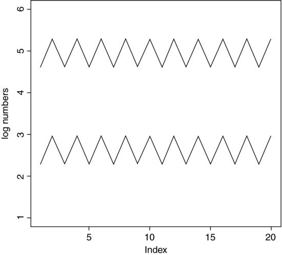
Now it is clear that both populations are equally variable. Note the change of scale, as specified using the ylim=c(1,6) option within the plot function (p. 193).
2.15.4 Harmonic mean
Consider the following problem. An elephant has a territory which is a square of side 2 km. Each morning, the elephant walks the boundary of this territory. He begins the day at a sedate pace, walking the first side of the territory at a speed of 1 km/hr. On the second side, he has sped up to 2 km/hr. By the third side he has accelerated to an impressive 4 km/hr, but this so wears him out, that he has to return on the final side at a sluggish 1 km/hr. So what is his average speed over the ground? You might say he travelled at 1, 2, 4 and 1 km/hr so the average speed is (1 + 2 + 4 + 1)/4 = 8/4 = 2 km/hr. But that is wrong. Can you see how to work out the right answer? Recall that velocity is defined as distance travelled divided by time taken. The distance travelled is easy: it is just 4 × 2 = 8 km. The time taken is a bit harder. The first edge was 2 km long, and travelling at 1 km/hr this must have taken 2 hr. The second edge was 2 km long, and travelling at 2 km/hr this must have taken 1 hr. The third edge was 2 km long and travelling at 4 km/hr this must have taken 0.5 hr. The final edge was 2 km long and travelling at 1 km/hr this must have taken 2 hr. So the total time taken was 2 + 1 + 0.5 + 2 = 5.5 hr. So the average speed is not 2 km/hr but 8/5.5 = 1.4545 km/hr. The way to solve this problem is to use the harmonic mean.
The harmonic mean is the reciprocal of the average of the reciprocals. The average of our reciprocals is:

The reciprocal of this average is the harmonic mean
In symbols, therefore, the harmonic mean,  (y-curl), is given by
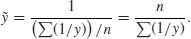
An R function for calculating harmonic means, therefore, could be
harmonic <- function (x) 1/mean(1/x)
and testing it on our elephant data gives
harmonic(c(1,2,4,1))
[1] 1.454545
2.15.5 Variance
A measure of variability is perhaps the most important quantity in statistical analysis. The greater the variability in the data, the greater will be our uncertainty in the values of parameters estimated from the data, and the less will be our ability to distinguish between competing hypotheses about the data.
The variance of a sample is measured as a function of ‘the sum of the squares of the difference between the data and the arithmetic mean’. This important quantity is called the ‘sum of squares’:
Naturally, this quantity gets bigger with every new data point you add to the sample. An obvious way to compensate for this is to measure variability as the average of the squared departures from the mean (the ‘mean square deviation’.). There is a slight problem, however. Look at the formula for the sum of squares, SS, above and ask yourself what you need to know before you can calculate it. You have the data, y, but the only way you can know the sample mean,  , is to calculate it from the data (you will never know in advance).
2.15.6 Degrees of freedom
To complete our calculation of the variance we need the degrees of freedom (d.f.). This important concept in statistics is defined as follows:

which is the sample size, n, minus the number of parameters, k, estimated from the data. For the variance, we have estimated one parameter from the data, , and so there are n − 1 degrees of freedom. In a linear regression, we estimate two parameters from the data, the slope and the intercept, and so there are n − 2 degrees of freedom in a regression analysis.
Variance is denoted by the lower-case Latin letter s squared: s2. The square root of variance, s, is called the standard deviation. We always calculate variance as
Consider the following data:
y <- c(13,7,5,12,9,15,6,11,9,7,12)
We need to write a function to calculate the sample variance: we call it variance and define it like this:
variance <- function(x) sum((x - mean(x))^2)/(length(x)-1)
and use it like this:
variance(y)
[1] 10.25455
Our measure of variability in these data, the variance, is thus 10.254 55. It is said to be an unbiased estimator because we divide the sum of squares by the degrees of freedom (n − 1) rather than by the sample size, n, to compensate for the fact that we have estimated one parameter from the data. So the variance is close to the average squared difference between the data and the mean, especially for large samples, but it is not exactly equal to the mean squared deviation. Needless to say, R has a built-in function to calculate variance called var:
var(y)
[1] 10.25455
2.15.7 Variance ratio test
How do we know if two variances are significantly different from one another? One of several sensible ways to do this is to carry out Fisher's F test, which is simply the ratio of the two variances (see p. 287). Here is a function to print the p value (p. 347) associated with a comparison of the larger and smaller variances:

The last line of our function works out the probability of getting an F ratio as big as vr or bigger by chance alone if the two variances were really the same, using the cumulative probability of the F distribution, which is an R function called pf. We need to supply pf with three arguments: the size of the variance ratio (vr), the number of degrees of freedom in the numerator (df1 = 9) and the number of degrees of freedom in the denominator (df2 = 9).
Here are some data to test our function. They are normally distributed random numbers but the first set has a variance of 4 and the second a variance of 16 (i.e. standard deviations of 2 and 4, respectively):
a <- rnorm(10,15,2)
b <- rnorm(10,15,4)
Here is our function in action:
variance.ratio(a,b)
[1] 0.01593334
We can compare our p with the p value given by the built-in function called var.test:
var.test(a,b)
F test to compare two variances
data: a and b
F = 0.1748, num df = 9, denom df = 9, p-value = 0.01593
alternative hypothesis: true ratio of variances is not equal to 1
95 percent confidence interval:
0.04340939 0.70360673
sample estimates:
ratio of variances
0.1747660
2.15.8 Using variance
Variance is used in two main ways: for establishing measures of unreliability (e.g. confidence intervals) and for testing hypotheses (e.g. Student's t test). Here we will concentrate on the former; the latter is discussed in Chapter 8.
Consider the properties that you would like a measure of unreliability to possess. As the variance of the data increases, what would happen to the unreliability of estimated parameters? Would it go up or down? Unreliability would go up as variance increased, so we would want to have the variance on the top (the numerator) of any divisions in our formula for unreliability:
What about sample size? Would you want your estimate of unreliability to go up or down as sample size, n, increased? You would want unreliability to go down as sample size went up, so you would put sample size on the bottom of the formula for unreliability (i.e. in the denominator):
Finally, consider the units in which unreliability is measured. What are the units in which our current measure is expressed? Sample size is dimensionless, but variance is based on the sum of squared differences, so it has dimensions of mean squared. So if the mean was a length in cm, the variance would be an area in cm2. This is an unfortunate state of affairs. It would make good sense to have the dimensions of the unreliability measure and of the parameter whose unreliability it is measuring the same. That is why all unreliability measures are enclosed inside a big square root term. Unreliability measures are called standard errors. What we have just worked out is the standard error of the mean,

where s2 is the variance and n is the sample size. There is no built-in R function to calculate the standard error of a mean, but it is easy to write one:
se <- function(x) sqrt(var(x)/length(x))
You can refer to functions from within other functions. Recall that a confidence interval (CI) is ‘t from tables times the standard error’:
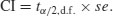
The R function qt gives the value of Student's t with 1 – α/2 = 0.975 and degrees of freedom d.f. = length(x)-1. Here is a function called ci95 which uses our function se to compute 95% confidence intervals for a mean:
ci95 <- function(x) {
t.value <- qt(0.975,length(x)-1)
standard.error <- se(x)
ci <- t.value*standard.error
cat("95 Confidence Interval = ", mean(x) -ci, "to ", mean(x) +ci,"\n") }
We can test the function with 150 normally distributed random numbers with mean 25 and standard deviation 3:
x <- rnorm(150,25,3)
ci95(x)
95% Confidence Interval = 24.76245 to 25.74469
If we were to repeat the experiment, we could be 95% certain that the mean of the new sample would lie between 24.76 and 25.74.
We can use the se function to investigate how the standard error of the mean changes with the sample size. First we generate one set of data from which we shall take progressively larger samples:
xv <- rnorm(30)
Now in a loop take samples of size 2, 3, 4, …, 30:
sem <- numeric(30)
sem[1] <- NA
for(i in 2:30) sem[i] <- se(xv[1:i])
plot(1:30,sem,ylim=c(0,0.8),
ylab="standard error of mean",xlab="sample size n",pch=16)
You can see clearly that as the sample size falls below about n = 15, so the standard error of the mean increases rapidly. The blips in the line are caused by outlying values being included in the calculations of the standard error with increases in sample size. The smooth curve is easy to compute: since the values in xv came from a standard normal distribution with mean 0 and standard deviation 1, so the average curve would be  , which we can add to our graph using lines:
lines(2:30,1/sqrt(2:30))
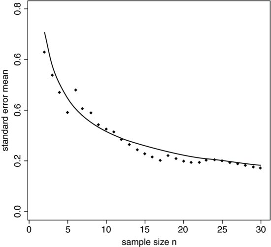
You can see that our single simulation captured the essence of the shape but was wrong in detail, especially for the samples with the lowest replication. However, our single sample was reasonably good for n > 24.
2.15.9 Deparsing: A graphics function for error bars
There is no function in the base package of R for drawing error bars on bar charts, although several contributed packages use the arrows function for this purpose (p. 204). Here is a simple, stripped-down function that is supplied with three arguments: the heights of the bars (yv), the lengths (up and down) of the error bars (z) and the labels for the bars on the x axis (nn).
The process of deparsing turns an unevaluated expression into a character string. One of the important uses of deparsing is in functions that produce output that you want to label with the particular names of the variables that were passed to the function. For instance, if the function is written in terms of a continuous response variable y and a categorical explanatory variable x, you might want to label the axes of a plot produced by the function with, say, clipping and biomass in place of x and y. For instance, if the function is written in terms of a continuous response variable yv, you might want to label the axes of a plot produced by the function with, say, biomass in place of yv. Inside the error.bars function, the barplot function uses the deparse function to create the appropriate text for ylab.
error.bars <- function(yv,z,nn){
xv <-
barplot(yv,ylim=c(0,(max(yv)+max(z))),names=nn,ylab=deparse(substitute(yv)
))
g=(max(xv)-min(xv))/50
for (i in 1:length(xv)) {
lines(c(xv[i],xv[i]),c(yv[i]+z[i],yv[i]-z[i]))
lines(c(xv[i]-g,xv[i]+g),c(yv[i]+z[i], yv[i]+z[i]))
lines(c(xv[i]-g,xv[i]+g),c(yv[i]-z[i], yv[i]-z[i]))
}}
Here is the error.bars function in action with the plant competition data (p. 426):
comp <- read.table("c:\\temp\\competition.txt",header=T)
attach(comp)
names(comp)
[1] "biomass" "clipping"
se <- rep(28.75,5)
labels <- as.character(levels(clipping))
ybar <- as.vector(tapply(biomass,clipping,mean))
Now invoke the function with the means, standard errors and bar labels:
error.bars(ybar,se,labels)

Here is a function to plot error bars on a scatterplot in both the x and y directions:
xy.error.bars <- function (x,y,xbar,ybar){
plot(x, y, pch=16, ylim=c(min(y-ybar),max(y+ybar)),
xlim=c(min(x-xbar),max(x+xbar)))
arrows(x, y-ybar, x, y+ybar, code=3, angle=90, length=0.1)
arrows(x-xbar, y, x+xbar, y, code=3, angle=90, length=0.1) }
We test it with these data:
x <- rnorm(10,25,5)
y <- rnorm(10,100,20)
xb <- runif(10)*5
yb <- runif(10)*20
xy.error.bars(x,y,xb,yb)
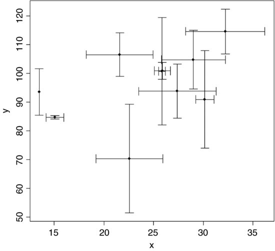
2.15.10 The switch function
When you want a function to do different things in different circumstances, then the switch function can be useful. Here we write a function that can calculate any one of four different measures of central tendency: arithmetic mean, geometric mean, harmonic mean or median (see pp. 115–119 for explanations of the separate functions). The character variable called measure should take one value of Mean, Geometric, Harmonic or Median; any other text will lead to the error message Measure not included. Alternatively, you can specify the number of the switch (e.g. 1 for Mean, 4 for Median).
central <- function(y, measure) {
switch(measure,
Mean = mean(y),
Geometric = exp(mean(log(y))),
Harmonic = 1/mean(1/y),
Median = median(y),
stop("Measure not included")) }
Note that you have to include the character strings in quotes as arguments to the function, but they must not be in quotes within the switch function itself.
central(rnorm(100,10,2),"Harmonic")
[1] 9.554712
central(rnorm(100,10,2),4)
[1] 10.46240
2.15.11 The evaluation environment of a function
When a function is called or invoked a new evaluation frame is created. In this frame the formal arguments are matched with the supplied arguments according to the rules of argument matching (below). The statements in the body of the function are evaluated sequentially in this environment frame.
The first thing that occurs in a function evaluation is the matching of the formal to the actual or supplied arguments. This is done by a three-pass process:
- Exact matching on tags. For each named supplied argument the list of formal arguments is searched for an item whose name matches exactly.
- Partial matching on tags. Each named supplied argument is compared to the remaining formal arguments using partial matching. If the name of the supplied argument matches exactly with the first part of a formal argument then the two arguments are considered to be matched.
- Positional matching. Any unmatched formal arguments are bound to unnamed supplied arguments, in order. If there is a … argument, it will take up the remaining arguments, tagged or not.
- If any arguments remain unmatched an error is declared.
Supplied arguments and default arguments are treated differently. The supplied arguments to a function are evaluated in the evaluation frame of the calling function. The default arguments to a function are evaluated in the evaluation frame of the function. In general, supplied arguments behave as if they are local variables initialized with the value supplied and the name of the corresponding formal argument. Changing the value of a supplied argument within a function will not affect the value of the variable in the calling frame.
2.15.12 Scope
The scoping rules are the set of rules used by the evaluator to find a value for a symbol. A symbol can be either bound or unbound. All of the formal arguments to a function provide bound symbols in the body of the function. Any other symbols in the body of the function are either local variables or unbound variables. A local variable is one that is defined within the function, typically by having it on the left-hand side of an assignment. During the evaluation process if an unbound symbol is detected then R attempts to find a value for it: the environment of the function is searched first, then its enclosure and so on until the global environment is reached. The value of the first match is then used.
2.15.13 Optional arguments
Here is a function called charplot that produces a scatterplot of x and y using solid red circles as the plotting symbols: there are two essential arguments (x and y) and two optional (pc and co) to control selection of the plotting symbol and its colour:
charplot <- function(x,y,pc=16,co="red"){
plot(y~x,pch=pc,col=co)}
The optional arguments are given their default values using = in the argument list. To execute the function you need only provide the vectors of x and y:
charplot(1:10,1:10)
to get solid red circles. You can get a different plotting symbol simply by adding a third argument
charplot(1:10,1:10,17)
which produces red solid triangles (pch=17). If you want to change only the colour (the fourth argument) then you have to specify the variable name because the optional arguments would not then be presented in sequence. So, for navy blue solid circles, you put:
charplot(1:10,1:10,co="navy")
To change both the plotting symbol and the colour you do not need to specify the variable names, so long as the plotting symbol is the third argument and the colour is the fourth:
charplot(1:10,1:10,15,"green")
This produces solid green squares. Reversing the optional arguments does not work:
charplot(1:10,1:10,"green",15)
(this uses the letter g as the plotting symbol and colour no. 15). If you specify both variable names, then the order does not matter:
charplot(1:10,1:10,co="green",pc=15)
This produces solid green squares despite the arguments being out of sequence.
2.15.14 Variable numbers of arguments (…)
Some applications are much more straightforward if the number of arguments does not need to be specified in advance. There is a special formal name … (triple dot) which is used in the argument list to specify that an arbitrary number of arguments are to be passed to the function. Here is a function that takes any number of vectors and calculates their means and variances:
many.means <- function (…) {
data <- list(…)
n <- length(data)
means <- numeric(n)
vars <- numeric(n)
for (i in 1:n) {
means[i] <- mean(data[[i]])
vars[i] <- var(data[[i]])
}
print(means)
print(vars)
invisible(NULL)
}
The main features to note are these. The function definition has … as its only argument. The ‘triple dot’ argument … allows the function to accept additional arguments of unspecified name and number, and this introduces tremendous flexibility into the structure and behaviour of functions. The first thing done inside the function is to create an object called data out of the list of vectors that are actually supplied in any particular case. The length of this list is the number of vectors, not the lengths of the vectors themselves (these could differ from one vector to another, as in the example below). Then the two output variables (means and vars) are defined to have as many elements as there are vectors in the parameter list. The loop goes from 1 to the number of vectors, and for each vector uses the built-in functions mean and var to compute the answers we require. It is important to note that because data is a list, we use double [[ ]] subscripts in addressing its elements.
Now try it out. To make things difficult we shall give it three vectors of different lengths. All come from the standard normal distribution (with mean 0 and variance 1) but x is 100 in length, y is 200 and z is 300 numbers long:
x <- rnorm(100)
y <- rnorm(200)
z <- rnorm(300)
Now we invoke the function:
many.means(x,y,z)

As expected, all three means (top row) are close to 0, and all three variances are close to 1 (bottom row).
You can use … to absorb some arguments into an intermediate function which can then be extracted by functions called subsequently. R has a form of lazy evaluation of function arguments in which arguments are not evaluated until they are needed (in some cases the argument will never be evaluated).
2.15.15 Returning values from a function
Often you want a function to return a single value (like a mean or a maximum), in which case you simply leave the last line of the function unassigned (i.e. there is no ‘gets arrow’ on the last line). Here is a function to return the median value of the parallel maxima (built-in function pmax) of two vectors supplied as arguments:
parmax <- function (a,b) {
c <- pmax(a,b)
median(c) }
Here is the function in action: the unassigned last line median(c) returns the answer
x <- c(1,9,2,8,3,7)
y <- c(9,2,8,3,7,2)
parmax(x,y)
[1] 8
If you want to return two or more variables from a function you should use return with a list containing the variables to be returned. Suppose we wanted the median value of both the parallel maxima and the parallel minima to be returned:
parboth <- function (a,b) {
c <- pmax(a,b)
d <- pmin(a,b)
answer <- list(median(c),median(d))
names(answer)[[1]] <- "median of the parallel maxima"
names(answer)[[2]] <- "median of the parallel minima"
return(answer) }
Here it is in action with the same x and y data as above:
parboth(x,y)
$"median of the parallel maxima"
[1] 8
$"median of the parallel minima"
[1] 2
The point is that you make the multiple returns into a list, then return the list. The provision of multi-argument returns (e.g. return(median(c),median(d)) in the example above) has been deprecated in R and a warning is given, as multi-argument returns were never documented in S, and whether or not the list was named differs from one version of S to another.
2.15.16 Anonymous functions
Here is an example of an anonymous function. It generates a vector of values but the function is not allocated a name (although the answer could be).
(function(x,y){ z <- 2* x^2 + y^2; x+y+z })(0:7, 1)
[1] 2 5 12 23 38 57 80 107
The function first uses the supplied values of x and y to calculate z, then returns the value of x + y + z evaluated for eight values of x (from 0 to 7) and one value of y (1). Anonymous functions are used most frequently with apply, tapply, sapply and lapply (p. 63).
2.15.17 Flexible handling of arguments to functions
Because of the lazy evaluation practised by R, it is very simple to deal with missing arguments in function calls, giving the user the opportunity to specify the absolute minimum number of arguments, but to override the default arguments if they want to. As a simple example, take a function plotx2 that we want to work when provided with either one or two arguments. In the one-argument case (only an integer x > 1 provided), we want it to plot z2 against z for z = 1 to x in steps of 1. In the second case, when y is supplied, we want it to plot y against z for z = 1 to x:
plotx2 <- function (x, y = z^2) {
z <- 1:x
plot(z,y,type="l") }
In many other languages, the first line would fail because z is not defined at this point. But R does not evaluate an expression until the body of the function actually calls for it to be evaluated (i.e. never, in the case where y is supplied as a second argument). Thus for the one-argument case we get a graph of z2 against z and in the two-argument case we get a graph of y against z (in this example, the straight line 1:12 vs. 1:12). We rescale the windows (width then height in inches) so that the graphs come out looking roughly square rather than elongated:
windows(7,4)
par(mfrow=c(1,2))
plotx2(12)
plotx2(12,1:12)
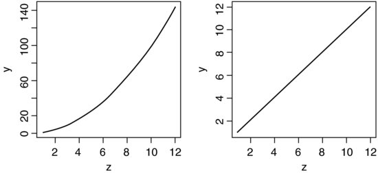
It is possible to access the actual (not default) expressions used as arguments inside the function. The mechanism is implemented via promises. You can find an explanation of promises by typing ?promise at the command prompt.
2.15.18 Structure of an object: str
Here is one of the simplest objects in R – a vector of length 7 containing real numbers:
(y <- seq(0.9,0.3,-0.1))
[1] 0.9 0.8 0.7 0.6 0.5 0.4 0.3
We can ask R about the structure of the object called y using str:
str(y)
num [1:7] 0.9 0.8 0.7 0.6 0.5 0.4 0.3
We discover that it is numeric (in both class and mode), a vector of length 7 [1:7], and (because the vector is short) we see all of the values listed. For longer vectors we would see the first few values, depending on what would fit on a single printed line (as affected by the number of decimal places displayed).
What about a slightly more complicated object? Here is a dataframe with two columns:
data <- read.table("c:\\temp\\spino.txt",header=T)
str(data)
'data.frame': 109 obs. of 2 variables:
$ condition: Factor w/ 5 levels "better","much.better",..: 4 1 1 4 4 4 1 5 4 1 …
$ treatment: Factor w/ 3 levels "drug.A","drug.B",..: 1 2 2 3 2 2 1 1 2 2 …
We learn that data is a dataframe with 109 rows and 2 columns, then we get detailed information on each of the columns in turn. The first is a variable called condition which is a factor with five levels (the first two levels of which (in alphabetical order) are better and much.better). The second variable is called treatment and is a factor with three levels. The numbers are the integer representations of the factor levels in the first 10 rows of the dataframe. Because we can see only factor levels 1 and 2, we would need to do more work to discover what factor level 4 of condition, or level 3 of treatment, actually represented:
levels(data$condition);levels(data$treatment)
[1] "better" "much.better" "much.worse" "no.change" "worse"
[1] "drug.A" "drug.B" "placebo"
We often want to know about the structure of model objects. Here is the simplest case, with a linear regression model (see p. 450 for details):
reg <- read.table("c:\\temp\\tannin.txt",header=T)
reg.model <- lm(growth~tannin,data=reg)
str(reg.model)
List of 12
$ coefficients : Named num [1:2] 11.76 -1.22
..- attr(*, "names")= chr [1:2] "(Intercept)" "tannin"
$ residuals : Named num [1:9] 0.244 -0.539 -1.322 2.894 -0.889 …
..- attr(*, "names")= chr [1:9] "1" "2" "3" "4" …
$ effects : Named num [1:9] -20.67 -9.42 -1.32 2.83 -1.01 …
..- attr(*, "names")= chr [1:9] "(Intercept)" "tannin" "" "" …
$ rank : int 2
$ fitted.values: Named num [1:9] 11.76 10.54 9.32 8.11 6.89 …
..- attr(*, "names")= chr [1:9] "1" "2" "3" "4" …
$ assign : int [1:2] 0 1
$ qr :List of 5
..$ qr : num [1:9, 1:2] -3 0.333 0.333 0.333 0.333 …
.. ..- attr(*, "dimnames")=List of 2
.. .. ..$ : chr [1:9] "1" "2" "3" "4" …
.. .. ..$ : chr [1:2] "(Intercept)" "tannin"
.. ..- attr(*, "assign")= int [1:2] 0 1
..$ qraux: num [1:2] 1.33 1.26
..$ pivot: int [1:2] 1 2
..$ tol : num 1e-07
..$ rank : int 2
..- attr(*, "class")= chr "qr"
$ df.residual : int 7
$ xlevels : Named list()
$ call : language lm(formula = growth ~ tannin, data = reg)
$ terms :Classes 'terms', 'formula' length 3 growth ~ tannin
.. ..- attr(*, "variables")= language list(growth, tannin)
.. ..- attr(*, "factors")= int [1:2, 1] 0 1
.. .. ..- attr(*, "dimnames")=List of 2
.. .. .. ..$ : chr [1:2] "growth" "tannin"
.. .. .. ..$ : chr "tannin"
.. ..- attr(*, "term.labels")= chr "tannin"
.. ..- attr(*, "order")= int 1
.. ..- attr(*, "intercept")= int 1
.. ..- attr(*, "response")= int 1
.. ..- attr(*, ".Environment")=<environment: R_GlobalEnv>
.. ..- attr(*, "predvars")= language list(growth, tannin)
.. ..- attr(*, "dataClasses")= Named chr [1:2] "numeric" "numeric"
.. .. ..- attr(*, "names")= chr [1:2] "growth" "tannin"
$ model :'data.frame': 9 obs. of 2 variables:
..$ growth: int [1:9] 12 10 8 11 6 7 2 3 3
..$ tannin: int [1:9] 0 1 2 3 4 5 6 7 8
..- attr(*, "terms")=Classes 'terms', 'formula' length 3 growth ~
tannin
.. .. ..- attr(*, "variables")= language list(growth, tannin)
.. .. ..- attr(*, "factors")= int [1:2, 1] 0 1
.. .. .. ..- attr(*, "dimnames")=List of 2
.. .. .. .. ..$ : chr [1:2] "growth" "tannin"
.. .. .. .. ..$ : chr "tannin"
.. .. ..- attr(*, "term.labels")= chr "tannin"
.. .. ..- attr(*, "order")= int 1
.. .. ..- attr(*, "intercept")= int 1
.. .. ..- attr(*, "response")= int 1
.. .. ..- attr(*, ".Environment")=<environment: R_GlobalEnv>
.. .. ..- attr(*, "predvars")= language list(growth, tannin)
.. .. ..- attr(*, "dataClasses")= Named chr [1:2] "numeric" "numeric"
.. .. .. ..- attr(*, "names")= chr [1:2] "growth" "tannin"
- attr(*, "class")= chr "lm"
There are 12 elements in the list representing the structure of this linear model object: coefficients, residuals, effects, rank, fitted values, assign, qr, residual degrees of freedom, xlevels, call, terms and model. Each of these, in turn, is broken down into components; for instance, the two coefficients are numbers (11.76 and –1.22), and their names are (Intercept) and tannin. You should work down the list and see if you can figure out why each row is an important part of the model.
For more complicated models, the structure is even more involved. Here is the structure of a generalized linear model with a binary response and binomial errors:
data <- read.table("c:\\temp\\spino.txt",header=T)
attach(data)
y <- factor(1+(condition=="better")+(condition=="much.better"))
model <- glm(y~treatment,binomial)
summary(model)
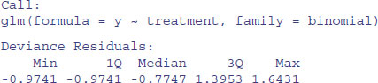

We have carried out a one-way analysis of deviance with a two-level response (improved or not) and a three-level factor as explanatory variable (treatment). There was no significant difference between drug.B and the placebo, nor between either of these and drug.A (the intercept). Here is the structure of the object called model:
str(model)
As you will see, this is a very large object, comprising a list with 30 components covering all aspects of the model: the coefficients, fitted values, effects plus all the details of the family and the model formula. I recommend you work your way slowly down the whole list and try to understand why each of the rows represents an essential piece of information about the model.
2.16 Writing from R to file
You often want to save an object that you have created in R.
2.16.1 Saving your work
To save your current R session, so that you can load it again later and continue your work where you left off, use save like this:
save(list = ls(all=TRUE), file= "c:\\temp\\session")
Then, on another occasion, when you want to restore the data, use load like this:
load(file= "c:\\temp\\session")
2.16.2 Saving history
It is very useful to be able to see all of the lines of R code that one has typed during a particular session. You may want to copy the lines into a text editor to make minor alterations, or you may simply want to paste multiple lines back into R to repeat certain operations. To see all of your lines of input code just type:
history(Inf)
This opens a window called R History through which you can scroll, highlight and copy using Ctrl+C. You could then open a new Untitled R Editor window (File > New Script) and paste the selected lines of code using Ctrl+V. Alternatively, you might want to save the entire history to file, for use on a subsequent occasion:
savehistory(file = "c:\\temp\\session18.txt")
To retrieve the history for use on another occasion use:
loadhistory(file = "c:\\temp\\session18.txt")
Then you can access it by history(Inf)in the new session.
2.16.3 Saving graphics
For speed and simplicity, you can click on a graph (the bar on top of the R Graphics Device goes darker blue) then press Ctrl+C (to copy the graph), then switch to a word processor and paste using Ctrl+V. For publication-quality graphics, however, you will want to save each figure in a separate file as a PDF or PostScript file. There are a great many options (see ?pdf and ?postscript for details) but the basics are very simple. Here we set the graphics device to produce a PDF:
pdf("c:\\temp\\fig1.pdf")
Now, any plot directives are sent to this file. To switch off writing graphics to file, type:
dev.off()
2.16.4 Saving data produced within R to disc
It is often convenient to generate numbers within R and then to use them somewhere else (in a spreadsheet, say). Here are 1000 random integers from a negative binomial distribution with mean mu=1.2 and clumping parameter or aggregation parameter (k) size = 1.0, that I want to save as a single column of 1000 rows in a file called nbnumbers.txt in the temp directory on the c: drive:
nbnumbers <- rnbinom(1000, size=1, mu=1.2)
There is general point to note here about the number and order of arguments provided to built-in functions like rnbinom. This function can have two of three optional arguments: size, mean (mu) and probability (prob) (see ?rnbinom). R knows that the unlabelled number 1000 refers to the number of numbers required because of its position, first in the list of arguments. If you are prepared to specify the names of the arguments, then the order in which they appear is irrelevant: rnbinom(1000, size=1, mu=1.2) and rnbinom(1000, mu=1.2, size=1) would give the same output. But if optional arguments are not labelled, then their order is crucial: so rnbinom(1000, 0.9, 0.6) is different from rnbinom(1000, 0.6, 0.9) because if there are no labels, then the second argument must be size and the third argument must be prob.
To export the numbers I use write like this, specifying that the numbers are to be output in a single column (i.e. with third argument 1 because the default is 5 columns):
write(nbnumbers,"c:\\temp\\nbnumbers.txt",1)
Sometimes you will want to save a table or a matrix of numbers to file. There is an issue here, in that the write function transposes rows and columns. It is much simpler to use the write.table function which does not transpose the rows and columns. Here is a matrix of 1000 rows and 100 columns made up of random integers from a Poisson distribution with mean 0.75:
xmat <- matrix(rpois(100000,0.75),nrow=1000)
write.table(xmat,"c:\\temp\\table.txt",col.names=F,row.names=F)
The function adds made-up row names and column names unless (as here) you specify otherwise. You have saved 1000 rows each of 100 Poisson random numbers with λ = 0.75.
Suppose that you have counted the number of different entries in the vector of negative binomial numbers (above):
nbtable <- table(nbnumbers)
nbtable

and you want write this output to a file. If you want to save both the counts and their frequencies in adjacent columns, use
write.table(nbtable,"c:\\temp\\table.txt",col.names=F,row.names=F)
but if you only want to export a single column of frequencies (445, 248, …) use
write.table(unclass(nbtable),"c:\\temp\\table.txt",col.names=F,row.names=F)
2.16.5 Pasting into an Excel spreadsheet
Writing a vector from R to the Windows Clipboard uses the function writeClipboard(x) where x is a single vector of characters, so you need to build up a spreadsheet in Excel by pasting (Ctrl+V) one column at a time. Remember that character strings in dataframes are converted to factors on input unless you protect them by as.is(name) on input. For example:
writeClipboard(as.character(factor.name))
Go into Excel and press Ctrl+V, and then back into R and type:
writeClipboard(as.character(numeric.variable))
Then go into Excel and press Ctrl+V in the second column, and so on.
2.16.6 Writing an Excel readable file from R
Suppose you want to transfer an entire dataframe called data to Excel (rather than one column, as above):
data <- read.table("c:\\temp\\worms.txt",header=T)
write.table(data,"clipboard",sep="\t",col.names=NA)
Then, in Excel, just press Ctrl+V or click on the Paste icon (the Clipboard). Your variable names will appear in the first row of the spreadsheet, with (unheaded) row numbers in the leftmost column.
2.17 Programming tips
- Know exactly what you are trying to achieve.
- Keep it simple.
- Clever is good, but clear is better.
- Test each line as you go along, to make sure it does what you want it to do.
- Put plenty of comments in the code, using # for documentation.
- Use variable names and function names that are self-explanatory.
- Do not use attach in programs.
- Use with, or refer to variables within named dataframes.
- Try different ways of doing the same thing, and select the fastest method.
- Use indents (tabs) to improve clarity of loops and if statements.
- Build up the program from small, independently tested functions.
- Stop tinkering once it works effectively.