3
Data Input
You can get numbers into R through the keyboard, from the Clipboard or from an external file. For a single variable of up to 10 numbers or so, it is probably quickest to type the numbers at the command line, using the concatenate function c like this:
y <- c (6,7,3,4,8,5,6,2)
For intermediate sized variables, you might want to enter data from the keyboard using the scan function. For larger data sets, and certainly for sets with several variables, you should make a dataframe externally (e.g. in a spreadsheet) and read it into R using read.table (p. 139).
3.1 Data input from the keyboard
The scan function is useful if you want to type (or paste) a few numbers into a vector called x from the keyboard:
x <-scan()
1:
At the 1: prompt type your first number, then press the Enter key. When the 2: prompt appears, type in your second number and press Enter, and so on. When you have put in all the numbers you need (suppose there are eight of them) then simply press the Enter key at the 9: prompt.
1: 6
2: 7
3: 3
4: 4
5: 8
6: 5
7: 6
8: 2
9:
Read 8 items
You can also use scan to paste in columns of numbers from the Clipboard. In the spreadsheet, highlight the column of numbers you want, then type Ctrl+C (the accelerator keys for Copy). Now go back into R. At the 1: prompt just type Ctrl+V (the accelerator keys for Paste) and the numbers will be scanned into the named variable (x in this example). You can then paste in another set of numbers, or press Return to complete data entry. If you try to read in a group of numbers from a row of cells in Excel, the characters will be pasted into a single multi-digit number (definitely not what is likely to have been intended). So, if you are going to paste numbers from Excel, make sure the numbers are in columns, not in rows, in the spreadsheet. If necessary, use Edit/Paste Special/Transpose in Excel to turn a row into a column before copying the numbers.
3.2 Data input from files
The easiest way to get data into R is to make your data into the shape of a dataframe before trying to read it into R. As explained in detail in Chapter 4, you should put all of the values of each variable into a single column, and put the name of the variable in row 1 (called the ‘header’ row). You will sometimes see the rows and the columns of the dataframe referred to as cases and fields respectively. In our terminology, the fields are the variables and the cases are rows.
Where you have text strings containing blanks (e.g. place names like ‘New Brighton’) then read.table is no good because it will think that ‘New’ is the value of one variable and ‘Brighton’ is another, causing the input to fail because the number of data items does not match the number of columns. In such cases, use a comma to separate the fields, and read the data from file using the function read.csv (the suffix .csv stands for ‘comma separated values’). The function read.csv2 is the variant for countries where a comma is used as the decimal point: in this case, a semicolon is the field separator.
3.2.1 The working directory
It is useful to have a working directory, because this makes accessing and writing files so much easier, since you do not need to type the (potentially long) path name each time. For instance, we can simplify data entry by using setwd to set the working directory to "c:\\temp":
setwd("c:\\temp")
To find out the name of the current working directory, use getwd() like this:
getwd()
[1] "c:/temp"
If you have not changed the working directory, then you will see something like this:
getwd()
[1] "C:/Documents and Settings/mjcraw/My Documents"
which is the working directory assumed by R when you start a new session. If you plan to switch back to the default working directory during a session, then it is sensible to save the long default path before you change it, like this:
mine<-getwd()
setwd("c:\\temp")
…
setwd(mine)
If you want to view file names from R, then use the dir function like this:
dir("c:\\temp")
To pick a file from a directory using the browser, invoke the file.choose function. This is most used in association with read.table if you have forgotten the name or the location of the file you want to read into a dataframe:
data<-read.table(file.choose(),header=T)
Just click on the file you want to read, and the contents will be assigned to the frame called data.
3.2.2 Data input using read.table
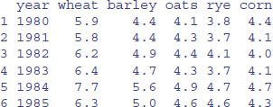
Here is an example of the standard means of data entry, creating a dataframe within R using read.table:
setwd("c:\\temp\\")
data <- read.table(yield.txt",header=T)
head(data)
You can save time by using read.delim, because then you can omit header=T:
data <- read.delim("yield.txt")
Or you could go the whole way down the labour-saving route and write your own text-minimizing function, which uses the paste function to add the suffix .txt as well as shortening the function name from read.table to rt like this:
rt <- function(x) read.table(paste("c:\\temp\\",x,".txt",sep=""),
header=TRUE)
Then simply type:
data <- rt("yields")
3.2.3 Common errors when using read.table
It is important to note that read.table would fail if there were any spaces in any of the variable names in row 1 of the dataframe (the header row, see p. 161), such as Field Name, Soil pH or Worm Density, or between any of the words within the same factor level (as in many of the field names). You should replace all these spaces by dots ‘.’ before saving the dataframe in Excel (use Edit/Replace with " " replaced by "." ). Now the dataframe can be read into R. There are three things to remember:
- The whole path and file name needs to be enclosed in double quotes: "c:\\abc.txt".
- header=T says that the first row contains the variable names (T stands for TRUE).
- Always use double \\ rather than \ in the file path definition.
The most common cause of failure is that the number of variable names (characters strings in row 1) does not match the number of columns of information. In turn, the commonest cause of this is that you have left blank spaces in your variable names:
state name population home ownership cars insurance
This is wrong because R expects seven columns of numbers when there are only five. Replace the spaces within the names by dots and it will work fine:
state.name population home.ownership cars insurance
The next most common cause of failure is that the data file contains blank spaces where there are missing values. Replace these blanks with NA in your spreadsheet before reading the file into R.
Finally, there can be problems when you are trying to read variables that consist of character strings containing blank spaces (as in files containing place names). You can use read.table so long as you export the file from the spreadsheet using commas to separate the fields, and you tell read.table that the separators are commas using sep="," (to override the default blanks or tabs (\t):
map <- read.table("c:\\temp\\bowens.csv",header=T,sep=",")
However, it is quicker and easier to use read.csv in this case (see below).
3.2.4 Separators and decimal points
The default field separator character in read.table is sep=" ". This separator is white space, which is produced by one or more spaces, one or more tabs \t, one or more newlines \n, or one or more carriage returns. If you do have a different separator between the variables sharing the same line (i.e. other than a tab within a.txt file) then there may well be a special read function for your case. Note that all the alternatives to read.table have the sensible default that header=TRUE (the first row contains the variable names):
- for comma-separated fields use read.csv("c:\\temp\\file.csv");
- for semicolon-separated fields read.csv2("c:\\temp\\file.csv");
- for tab-delimited fields with decimal points as a commas, use read.delim2("c:\\temp\\file.txt").
You would use comma or semicolon separators if you had character variables that might contain one or more blanks (e.g. country names like ‘United Kingdom’ or ‘United States of America’).
If you want to specify row.names then one of the columns of the dataframe must be a vector of unique row names. This can be a single number giving the column of the table which contains the row names, or character string giving the variable name of the table column containing the row names (see p. 176). Otherwise, if row.names is missing, rows numbers are generated automatically on the left of the dataframe.
The default behaviour of read.table is to convert character variables into factors. If you do not want this to happen (you want to keep a variable as a character vector) then use as.is to specify the columns that should not be converted to factors:
murder <- read.table("c:\\temp\\murders.txt",header=T,as.is="region")
3.2.5 Data input directly from the web
You will typically use read.table to read data from a file, but the function also works for complete URLs. In computing, URL stands for ‘universal resource locator’, and is a specific character string that constitutes a reference to an Internet resource, combining domain names with file path syntax, where forward slashes are used to separate folder and file names:
data2 <- read.table
("http://www.bio.ic.ac.uk/research/mjcraw/therbook/data/cancer.txt",
header=T)
head(data2)
3.3 Input from files using scan
For dataframes, read.table is superb. But look what happens when you try to use read.table with a more complicated file structure:
read.table("c:\\temp\\rt.txt")
Error in scan(file, what, nmax, sep, dec, quote, skip, nlines, na.strings
line 1 did not have 4 elements
It simply cannot cope with lines having different numbers of fields. However, scan and readLines come into their own with these complicated, non-standard files.
The scan function reads data into a list when it is used to read from a file. It is much less friendly for reading dataframes than read.table, but it is substantially more flexible for tricky or non-standard files.
By default, scan assumes that you are inputting double precision numbers. If not, then you need to use the what argument to explain what exactly you are inputting (e.g. ‘character’, ‘logical’, ‘integer’, ‘complex’ or ‘list’). The file name is interpreted relative to the current working directory (given by getwd()), unless you specify an absolute path. If what is itself a list, then scan assumes that the lines of the data file are records, each containing one or more items and the number of fields on that line is given by length(what).
By default, scan expects to read space-delimited or tab-delimited input fields. If your file has separators other than blank spaces or tab markers (\t), then you can specify the separator option (e.g. sep=",") to specify the character which delimits fields. A field is always delimited by an end-of-line marker unless it is quoted. If sep is the default (""), the character \ in a quoted string escapes the following character, so quotes may be included in the string by escaping them ("she.said \"What!\".to.him"). If sep is non-default, the fields may be quoted in the style of .csv files where separators inside quotes ('' or "") are ignored and quotes may be put inside strings by doubling them. However, if sep = "\n" it is assumed by default that one wants to read entire lines verbatim.
With scan, you will often want to skip the header row (because this contains variable names rather than data). The option for this is skip = 1 ( you can specify any number of lines to be skipped before beginning to read data values). If a single record occupies more than one line of the input file then use the option multi.line =TRUE.
3.3.1 Reading a dataframe with scan
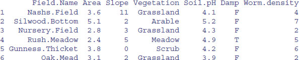
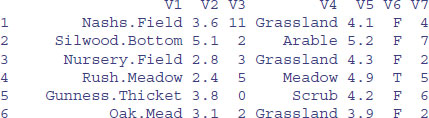
To illustrate the issues involved with scan, and to demonstrate why read.table is the preferred way of reading data into dataframes, we use scan to input the worms dataframe (for details, see Chapter 4). We want to skip the first row because that is a header containing the variable names, so we specify skip = 1. There are seven columns of data, so we specify seven fields of character variables "" in the list supplied to what:
scan("t:\\data\\worms.txt",skip=1,what=as.list(rep("",7)))

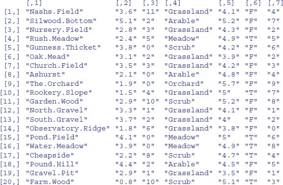
As you can see, scan has created a list of seven vectors of character string information. To convert this list into a dataframe, we use the as.data.frame function which turns the lists into columns in the dataframe (so long as the columns are all the same length):
data <-
as.data.frame(scan("t:\\data\\worms.txt",skip=1,what=as.list(rep("",7))))
In its present form, the variable names manufactured by scan are ridiculously long, so we need to replace them with the original variable names that are in the first row of the file. For this we can use scan again, but specify that we want to read only the first line, by specifying nlines=1 and removing the skip option:
header <- unlist(scan("t:\\data\\worms.txt",nlines=1,what=as.list
(rep("",7))))
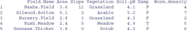
Now, we replace the manufactured names by the correct variable names in data:
names(data)<-header
head(data)
This has produced the right result, but you can see why you would want to use read.table rather than scan for reading dataframes.
3.3.2 Input from more complex file structures using scan
Here is an image of a file containing information on the identities of the neighbours of five individuals from a population: the first individual has one neighbour (number 138), the second individual has two neighbours (27 and 44), the third individual has four neighbours, and so on.
138
27 44
19 20 345 48
115 2366
59
See if you can figure out why the following three different readings of the same file rt.txt produce such different objects; the first has 10 items, the second 5 items and the third 20 items:
scan("c:\\temp\\rt.txt")
Read 10 items
[1] 138 27 44 19 20 345 48 115 2366 59
scan("c:\\temp\\rt.txt",sep="\n")
Read 5 items
[1] 138 2744 192034548 1152366 59
scan("c:\\temp\\rt.txt",sep="\t")
Read 20 items
[1] 138 NA NA NA 27 44 NA NA 19 20 345 48 115
[14] 2366 NA NA 59 NA NA NA
The only difference between the three calls to scan is in the specification of the separator. The first uses the default which is blanks or tabs (the 10 items are the 10 numbers that we are interested in, but information about their grouping has been lost). The second uses the new line "\n" control character as the separator (the contents of each of the five lines have been stripped out and trimmed to create meaningless numbers, except for 138 and 59 which were the only numbers on their respective lines). The third uses tabs "\t" as separators (we have no information on lines, but at least the numbers have retained their integrity, and missing values (NA) have been used to pad out each line to the same length, 4. To get the result we want we need to use the information on the number of lines from method 2 and the information on the contents of each line from method 3. The first step is easy:
length(scan("c:\\temp\\rt.txt",sep="\n"))
Read 5 items
[1] 5
So we have five lines of information in this file. To find the number of items per line were divide the total number of items
length(scan("c:\\temp\\rt.txt",sep="\t"))
Read 20 items
[1] 20
by the number of lines: 20 / 5 = 4. To extract the information on each line, we want to take a line at a time, and extract the missing values (i.e. remove the NAs). So, for line 1 this would be
scan("c:\\temp\\rt.txt",sep="\t")[1:4]
Read 20 items
[1] 138 NA NA NA
then, to remove the NA we use na.omit, to remove the Read 20 items we use quiet=T and to leave only the numerical value we use as.numeric:
as.numeric(na.omit(scan("c:\\temp\\rt.txt",sep="\t",quiet=T)[1:4]))
[1] 138
To complete the job, we need to apply this logic to each of the five lines in turn, to produce a list of vectors of variable lengths (1, 2, 4, 2 and 1):
sapply(1:5, function(i)
as.numeric(na.omit(
scan("c:\\temp\\rt.txt",sep="\t",quiet=T)[(4*i-3):
(4*i)])))
[[1]]
[1] 138
[[2]]
[1] 27 44
[[3]]
[1] 19 20 345 48
[[4]]
[1] 115 2366
[[5]]
[1] 59
That was about as complicated a procedure as you are likely to encounter in reading information from a file. In hindsight, we might have created the data as a dataframe with missing values explicitly added to the rows that had less than four numbers. Then a single read.table statement would have been enough.
3.4 Reading data from a file using readLines
An alternative is to use readLines instead of scan. Here is a repeat of the example of reading the worms dataframe (above).
3.4.1 Input a dataframe using readLines
line<-readLines("c:\\temp\\worms.txt")
line
[1] "Field.Name\tArea\tSlope\tVegetation\tSoil.pH\tDamp\tWorm.density"
[2] "Nashs.Field\t3.6\t11\tGrassland\t4.1\tFALSE\t4"
[3] "Silwood.Bottom\t5.1\t2\tArable\t5.2\tFALSE\t7"
[4] "Nursery.Field\t2.8\t3\tGrassland\t4.3\tFALSE\t2"
[5] "Rush.Meadow\t2.4\t5\tMeadow\t4.9\tTRUE\t5"
[6] "Gunness.Thicket\t3.8\t0\tScrub\t4.2\tFALSE\t6"
[7] "Oak.Mead\t3.1\t2\tGrassland\t3.9\tFALSE\t2"
[8] "Church.Field\t3.5\t3\tGrassland\t4.2\tFALSE\t3"
[9] "Ashurst\t2.1\t0\tArable\t4.8\tFALSE\t4"
[10] "The.Orchard\t1.9\t0\tOrchard\t5.7\tFALSE\t9"
[11] "Rookery.Slope\t1.5\t4\tGrassland\t5\tTRUE\t7"
[12] "Garden.Wood\t2.9\t10\tScrub\t5.2\tFALSE\t8"
[13] "North.Gravel\t3.3\t1\tGrassland\t4.1\tFALSE\t1"
[14] "South.Gravel\t3.7\t2\tGrassland\t4\tFALSE\t2"
[15] "Observatory.Ridge\t1.8\t6\tGrassland\t3.8\tFALSE\t0"
[16] "Pond.Field\t4.1\t0\tMeadow\t5\tTRUE\t6"
[17] "Water.Meadow\t3.9\t0\tMeadow\t4.9\tTRUE\t8"
[18] "Cheapside\t2.2\t8\tScrub\t4.7\tTRUE\t4"
[19] "Pound.Hill\t4.4\t2\tArable\t4.5\tFALSE\t5"
[20] "Gravel.Pit\t2.9\t1\tGrassland\t3.5\tFALSE\t1"
[21] "Farm.Wood\t0.8\t10\tScrub\t5.1\tTRUE\t3"
Each line has become a single character string. As you can see, we shall need to strip out all of the tab marks (\t), thereby separating the data entries and creating seven columns of information. The function for this is strsplit:
db<-strsplit(line,"\t")
db

and so on for 21 elements of the list. The new challenge is to get this into a form that we can turn into a dataframe. The first issue is to get rid of the list structure using the unlist function:
bb<-unlist(db)

and so on up to 147 items. We need to give this vector dimensions: the seven variable names come first, so the appropriate dimensionality is (7,21):
dim(bb)<-c(7,21)
bb

and so on for 21 rows. This is closer, but the rows and columns are the wrong way around. We need to transpose this object and drop the first row (because this is the header row containing the variable names):
t(bb)[-1,]
That's more like it. Now the function as.data.frame should work:
frame<-as.data.frame(t(bb)[-1,])
head(frame)
All we need to do now is add in the variable names: these are in the first row of the transpose of the object called bb (above):
names(frame)<-t(bb)[1,]
head(frame)
The complexity of this procedure makes you appreciate just how useful the function read.table really is.
3.4.2 Reading non-standard files using readLines
Here is a repeat of the example of the neighbours file that we analysed using scan on p. 141:
readLines("c:\\temp\\rt.txt")
[1] "138\t\t\t" "27\t44\t\t" "19\t20\t345\t48" "115\t2366\t\t"
[5] "59\t\t\t"
The readLines function had produced a vector of length 5 (one element for each row in the file), with the contents of each row reduced to a single character string (including the literal tab markers \t). We need to spit this up within the lines using strsplit: we split first on the tabs, then on the new lines in order to see the distinction:
strsplit(readLines("c:\\temp\\rt.txt"),"\t")
[[1]]
[1] "138" "" ""
[[2]]
[1] "27" "44" ""
[[3]]
[1] "19" "20" "345" "48"
[[4]]
[1] "115" "2366" ""
[[5]]
[1] "59" "" ""
strsplit(readLines("c:\\temp\\rt.txt"),"\n")
[[1]]
[1] "138\t\t\t"
[[2]]
[1] "27\t44\t\t"
[[3]]
[1] "19\t20\t345\t48"
[[4]]
[1] "115\t2366\t\t"
[[5]]
[1] "59\t\t\t"
The split by tab markers is closest to what we want to achieve, so we shall work on that. First, turn the character strings into numbers:
rows<-lapply(strsplit(readLines("c:\\temp\\rt.txt"),"\t"),as.numeric)
rows
[[1]]
[1] 138 NA NA
[[2]]
[1] 27 44 NA
[[3]]
[1] 19 20 345 48
[[4]]
[1] 115 2366 NA
[[5]]
[1] 59 NA NA
Now all that we need to do is to remove the NAs from each of the vectors:
sapply(1:5, function(i) as.numeric(na.omit(rows[[i]])))
[[1]]
[1] 138
[[2]]
[1] 27 44
[[3]]
[1] 19 20 345 48
[[4]]
[1] 115 2366
[[5]]
[1] 59
Both scan and readLines were fiddly, but they got what we were looking for in the end. You will need a lot of practice before you appreciate when to use scan and when to use readLines. Writing lists to files is tricky (see p. 82 for an explanation of the options available).
3.5 Warnings when you attach the dataframe
Suppose that you read a file from data, then attach it:
murder <- read.table("c:\\temp\\murders.txt",header=T,as.is="region")
The following warning will be produced if your attach function causes a duplication of one or more names:
attach(murder)
The following object(s) are masked _by_ .GlobalEnv:
murder
The reason in the present case is that we have created a dataframe called murder and attached a variable from this dataframe which is also called murder. This shows the cause of the problem: the dataframe name and the third variable name are identical:
head(murder)
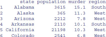
This ambiguity might cause difficulties later. A much better plan is to give the dataframe a unique name (like murders, for instance). We use the attach function so that the variables inside a dataframe can be accessed directly by name. Technically, this means that the dataframe is attached to the R search path, so that the dataframe is searched by R when evaluating a variable. We could tabulate the numbers of murders by region, for instance:
table(region)

If we had not attached the dataframe, then we would have had to specify the name of the dataframe first like this:
table(murder$region)
3.6 Masking
You may have attached the same dataframe twice. Alternatively, you may have two dataframes attached that have one or more variable names in common. The commonest cause of masking occurs with simple variable names like x and y. It is very easy to end up with multiple variables of the same name within a single session that mean totally different things. The warning after using attach should alert you to the possibility of such problems. If the vectors sharing the same name are of different lengths, then R is likely to stop you before you do anything too silly, but if the vectors are of the same length then you run the serious risk of fitting the wrong explanatory variable (e.g. fitting the wrong one from two vectors both called x) or having the wrong response variable (e.g. from two vectors both called y). The moral is:
- use longer, more self-explanatory variable names;
- do not calculate variables with the same name as a variable inside a dataframe;
- always detach dataframes once you have finished using them;
- remove calculated variables once you are finished with them (rm; see p. 10).
The best practice, however, is not to use attach in the first place, but to use functions like with instead (see p. 113). If you get into a real tangle, it is often easiest to quit R and start another R session.
The opposite problem occurs when you assign values to an existing variable name (perhaps by accident); the original contents of the name are lost.
z <- 10
…
…
z <- 2.5
Now, z is 2.5 and there is no way to retrieve the original value of 10.
3.7 Input and output formats
Formatting is controlled using escape sequences, typically within double quotes:
\n newline
\r carriage return
\t tab character
\b backspace
\a bell
\f form feed
\v vertical tab
Here is an example of the cat function. The default produces the output on the computer screen, but you can save the output to file using a file=file.name argument:
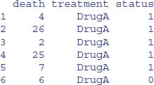
data<-read.table("c:\\temp\\catdata.txt",header=T)
attach(data)
names(data)
[1] "y" "soil"
model<-lm(y~soil)
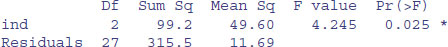
Suppose that you wanted to produce a slightly different layout for the ANOVA table than that produced by summary.aov(model):
summary.aov(model)
with the sum of squares column before the degrees of freedom column, plus a row for the total sum of squares, different row labels, and no p value, like this:
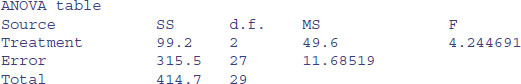
First, extract the necessary numbers from the summary.aov object:
df1<-unlist(summary.aov(model)[[1]] [1])[1]
df2<-unlist(summary.aov(model)[[1]] [1])[2]
ss1<-unlist(summary.aov(model)[[1]] [2])[1]
ss2<-unlist(summary.aov(model)[[1]] [2])[2]
Here is the R code to produce the ANOVA table, using cat with multiple tabs ("\t\t") and single new-line markers ("\n") at the end of each line:
{cat("ANOVA table","\n")
cat("Source","\t\t","SS","\t","d.f.","\t","MS","\t\t","F","\n")
cat("Treatment","\t",ss1,"\t",df1,"\t",ss1/df1,"\t\t",
(ss1/df1)/(ss2/df2),"\n")
cat("Error","\t\t",ss2,"\t",df2,"\t",ss2/df2,"\n")
cat("Total","\t\t",ss1+ss2,"\t",df1+df2,"\n")}
Note the use of curly brackets to group the five cat functions into a single print object.
3.8 Checking files from the command line
It can be useful to check whether a given filename exists in the path where you think it should be. The function is file.exists and is used like this:
file.exists("c:\\temp\\Decay.txt")
[1] TRUE
For more on file handling, see ?files.
3.9 Reading dates and times from files
You need to be very careful when dealing with dates and times in any sort of computing. R has a robust system for working with dates and times, but it takes some getting used to. Typically, you will read dates and times into R as character strings, then convert them into dates and times using the strptime function to explain exactly what the elements of the character string mean (e.g. which are the days, which are the months, what are the separators, and so on; see p. 103 for an explanation of the formats supported).
3.10 Built-in data files
There are many built-in data sets within the datasets package of R. You can see their names by typing:
data()
To see the data sets in extra installed packages as well, type:
data(package = .packages(all.available = TRUE))
You can read the documentation for a particular data set with the usual query:
?lynx
Many of the contributed packages contain data sets, and you can view their names using the try function. This evaluates an expression and traps any errors that occur during the evaluation. The try function establishes a handler for errors that uses the default error handling protocol:
try(data(package="spatstat"));Sys.sleep(3)
try(data(package="spdep"));Sys.sleep(3)
try(data(package="MASS"))
where try is a wrapper to run an expression that might fail and allow the user's code to handle error recovery, so this would work even if one of the packages was missing.
Built-in data files can be attached in the normal way; then the variables within them accessed by their names:
attach(OrchardSprays)
decrease
3.11 File paths
There are several useful R functions for manipulating file paths. A file path is a character string that looks something like this:
c:\\temp\\thesis\\chapter1\\data\\problemA
and you would not want to type all of that every time you wanted to read data or save material to file. You can set the default file path for a session using the current working directory:
setwd("c:\\temp\\thesis\\chapter1\\data")
The basename function removes all of the path up to and including the last path separator (if any):
basename("c:\\temp\\thesis\\chapter1\\data\\problemA")
[1] "problemA"
The dirname function returns the part of the path up to but excluding the last path separator, or "." if there is no path separator:
dirname("c:\\temp\\thesis\\chapter1\\data\\problemA")
[1] "c:/temp/thesis/chapter1/data"
Note that this function returns forward slashes as the separator, replacing the double backslashes.
Suppose that you want to construct the path to a file from components in a platform-independent way. The file.path function does this very simply:
A <- "c:"
B <- "temp"
C <- "thesis"
D <- "chapter1"
E <- "data"
F <- "problemA"
file.path(A,B,C,D,E,F)
[1] "c:/temp/thesis/chapter1/data/problemA"
The default separator is platform-dependent (/ in the example above, not \, but you can specify the separator (fsep) like this:
file.path(A,B,C,D,E,F,fsep="\\")
[1] "c:\\temp\\thesis\\chapter1\\data\\problemA"
3.12 Connections
Connections are ways of getting information into and out of R, such as your keyboard and your screen. The three standard connections are known as stdin() for input, stdout() for output, and stderr() for reporting errors. They are text-mode connections of class terminal which cannot be opened or closed, and are read-only, write-only and write-only respectively. When R is reading a script from a file, the file is the ‘console’: this is traditional usage to allow in-line data.
Functions to create, open and close connections include file, url, gzfile, bzfile, xzfile, pipe andsocketConnction. The intention is that file and gzfile can be used generally for text input (from files and URLs) and binary input, respectively. The functions file, pipe, fifo, url, gzfile, bzfile, xzfile, unz and socketConnection return a connection object which inherits from class connection: isOpen returns a logical value, indicating whether the connection is currently open; isIncomplete returns a logical value, indicating whether the last read attempt was blocked, or for an output text connection whether there is unflushed output. The functions are used like this:
file(description = "", open = "", blocking = TRUE,
encoding = getOption("encoding"), raw = FALSE)
For file the description is a path to the file to be opened or a complete URL, or "" (the default) or "clipboard". You can use file with description = "clipboard" in modes "r" and "w" only. There is a 32Kb limit on the text to be written to the Clipboard. This can be raised by using, for example, file("clipboard-128") to give 128Kb. For gzfile the description is the path to a file compressed by gzip: it can also open for reading uncompressed files and those compressed by bzip2, xz or lzma. For bzfile the description is the path to a file compressed by bzip2. For xzfile the description is the path to a file compressed by xz or lzma. A maximum of 128 connections can be allocated (not necessarily open) at any one time.
Not all modes are applicable to all connections: for example, URLs can only be opened for reading. Only file and socket connections can be opened for both reading and writing. For compressed files, the type of compression involves trade-offs: gzip, bzip2 and xz are successively less widely supported, need more resources for both compression and decompression, and achieve more compression (although individual files may buck the general trend). Typical experience is that bzip2 compression is 15% better on text files than gzip compression, and xz with maximal compression 30% better. With current computers decompression times even with compress = 9 are typically modest, and reading compressed files is usually faster than uncompressed ones because of the reduction in disc activity.
3.13 Reading data from an external database
Open Data Base Connectivity (ODBC) provides a standard software interface for accessing database management systems (DBMS) that is independent of programming languages, database systems and operating systems. Thus, any application can use ODBC to query data from a database, regardless of the platform it is on or the DBMS it uses. ODBC accomplishes this by using a driver as a translation layer between the application and the DBMS. The application thus only needs to know ODBC syntax, and the driver can then pass the query to the DBMS in its native format, returning the data in a format that the application can understand. Communication with the database uses SQL (‘Structured Query Language’).
The example we shall use is called Northwind. This is a relational database that is downloaded for Access from Microsoft Office, and which is used in introductory texts on SQL (e.g. Kauffman et al., 2001). The database refers to a fictional company that operates as a food wholesaler. You should download the database from http://office.microsoft.com. There are many related tables in the database, each with its unique row identifier (ID):
- Categories: 18 rows describing the categories of goods sold (from baked goods to oils) including Category name as well as Category.ID
- Products: 45 rows with details of the various products sold by Northwind including CategoryID (as above) and Product.ID
- Suppliers: 10 rows with details of the firms that supply goods to Northwind
- Shippers: 3 rows with details of the companies that ship goods to customers
- Employees: 9 rows with details of the people who work for Northwind
- Customers: 27 rows with details of the firms that buy goods from Northwind
- Orders: empty rows with orders from various customers tagged by OrderID
- Order Details: 2155 rows containing one to many rows for each order (typically 2 or 3 rows per order), each row containing the product, number required, unit price and discount, as well as the (repeated) OrderID
- Order Status: four categories – new, invoiced, shipped or completed
- Order Details: empty rows
- Order Details Status: six categories – none, no stock, back-ordered, allocated, invoiced and shipped
- Inventory: details of the 45 products held on hand and reordered.
The tables are related to one another like this:
- Orders and Order Details are related by a unique OrderID;
- Categories and Products are related by a unique CategoryID;
- Employees and Orders are linked by a unique EmployeeID;
- Products and Order Details are linked by a unique ProductID;
- and so on.
3.13.1 Creating the DSN for your computer
To analyse data from these tables in R we need first to set up a channel through which to access the information. Outside R, you need to give your computer a data source name (DSN) to associate with the Access database. This is a bit fiddly, but here is how to do it in Windows 7, assuming you have Microsoft Office 2010 and have already downloaded the Northwind database (you will need to figure out the equivalent directions for Mac or Linux, or if you are not using Office 2010):
- Go to Computer, click on Drive C: and then scroll down and click on the Windows folder.
- Scroll down and click on SysWOW64.
- Scroll way down and double-click on odbcad32.exe.
- The ODBC Data Source Administrator window should appear.
- Click on the Add button.
- Scroll down to Microsoft Access Driver (*.mdb,*.accdb) and click on Finish.
- The ODBC Microsoft Access Setup window should appear.
- In the top box write “northwind” (with no quote marks).
- In the second box write “example” (with no quote marks).
- Then, under Database, click on Select.
- Browse through the directory to the place where you put Northwind.accdb.
- Accept and you should see “northwind” has been added to the ODBC Data Source list.
- Click on OK at the bottom of the window to complete the task.
Fortunately, you need only do this once. Now you can access Northwind from R.
3.13.2 Setting up R to read from the database
If you have not done so already, you will need to obtain the package called RODBC that provides access to databases from within R. So start up R (run as administrator) then type:
install.packages("RODBC")
Open the library and tell R the name of the channel through which it can access the database (as set up in the previous section) using the function odbcConnect:
library(RODBC)
channel <- odbcConnect("northwind")
You communicate with the database from R using SQL. The syntax is very simple. You create a dataframe in R from a table (or more typically from several related tables) in the database using the function sqlQuery like this:
new.datatframe <- sqlQuery(channel, query)
The channel is defined using the odbcConnect function, as shown above. The skill is in creating the (often complicated) character string called query. The key components of an SQL query are:
| SELECT | a list of the variables required (or * for all variables) |
| FROM | the name of the table containing these variables |
| WHERE | specification of which rows of the table(s) are required |
| JOIN | the tables to be joined and the variables on which to join them |
| GROUP BY | columns with factors to act as grouping levels |
| HAVING | conditions applied after grouping |
| ORDER BY | sorted on which variables |
| LIMIT | offsets or counts |
The simplest cases require only SELECT and FROM.
Let us start by creating a dataframe in R called containing all of the variables (*) and rows from the table called Categories in Northwind:
query <- "SELECT * FROM Categories"
stock <- sqlQuery(channel, query)
This is what the R dataframe looks like – there are just two fields ID and Category:
stock

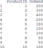
More usually, you will want to select only some of the variables from a table. From the table called Inventory, for example, we might want to extract only ProductID and OnHand to make a dataframe called quantities:
query <- "SELECT ProductID,OnHand FROM Inventory"
quantities <- sqlQuery(channel, query)
head(quantities,10)
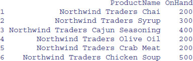
This would be a lot more informative if we could see the product names rather than their ID numbers. The names are in a different table called Products. We need to relate the two tables Inventory and Produces. The variable relating the two tables is ProductID from Inventory and ID from Products. The convention is to expand the variable names by adding the table name in front of the variable name, and separating the two names by a full stop, like this:
query <- "SELECT Products.ProductName, Inventory.OnHand FROM
Inventory INNER JOIN Products ON Inventory.ProductID = Products.ID "
quantities <- sqlQuery(channel, query)
head(quantities,10)

So that is how we relate two tables.
The next task is data selection. This involves the WHERE command in SQL. Here are the cases with more than 150 items on hand:
query <- "SELECT Products.ProductName, Inventory.OnHand FROM
Inventory INNER JOIN Products ON Inventory.ProductID = Products.ID
WHERE Inventory.OnHand > 150 "
supply <- sqlQuery(channel, query)
head(supply,10)
Using WHERE with text is more challenging because the text needs to be enclosed in quotes and quotes are always tricky in character strings. The solution is to mix single and double quotes to paste together the query you want:
name <- "NWTDFN-14"
query <- paste("SELECT ProductName FROM Products WHERE
ProductCode='",name,"'",sep="")
code <- sqlQuery(channel, query)
head(code,10)
ProductName
1 Northwind Traders Walnuts
This is what the query looks like as a single character string:
query
[1] "SELECT ProductName FROM Products WHERE ProductCode='NWTDFN-14'"
You will need to ponder this query really hard in order to see why we had to do what we did to select the ProductCode on the basis of its being "NWTDFN-14". The problem is that quotes must be part of the character string that forms the query, but quotes generally mark the end of a character string. There is another example of selecting records on the basis of character strings on p. 197 where we use data from a large relational database to produce species distribution maps.
While you have the Northwind example up and running, you should practise joining together three tables, and use some of the other options for selecting records, using LIKE with wildcards * (e.g. WHERE Variable.name LIKE "Product*").