Chapter 6
Tables
The alternative to using graphics is to summarize your data in tabular form. Broadly speaking, if you want to convey detail use a table, and if you want to show effects then use graphics. You are more likely to want to use a table to summarize data when your explanatory variables are categorical (such as people's names, or different commodities) than when they are continuous (in which case a scatterplot is likely to be more informative; see p. 189).
There are two very important functions that you need to distinguish:
- table for counting things;
- tapply for averaging things, and applying other functions across factor levels.
6.1 Tables of counts
The table function is perhaps the most useful of all the simple vector functions, because it does so much work behind the scenes. We have a vector of objects (they could be numbers or character strings) and we want to know how many of each is present in the vector. Here are 1000 integers from a Poisson distribution with mean 0.6:
counts<-rpois(1000,0.6)
We want to count up all of the zeros, ones, twos, and so on. A big task, but here is the table function in action:
table(counts)
counts
0 1 2 3 4 5
539 325 110 24 1 1
There were 539 zeros, 325 ones, 110 twos, 24 threes, 1 four, 1 five and nothing larger than 5. That is a lot of work (imagine tallying them for yourself). The function works for characters as well as for numbers, and for multiple classifying variables:
infections<-read.table("c:\\temp\\disease.txt",header=T)
attach(infections)
head(infections)
status gender
1 clear male
2 clear male
3 clear male
4 clear male
5 clear male
6 clear male
and so on for 1000 rows. You want to know how many males and females were infected and how many were clear of infection:
table(status,gender)
gender
status females male
clear 284 515
infected 53 68
If you want the genders as the rows rather than the columns, then put gender first in the argument list to table:
table(gender,status)
status
gender clear infected
females 284 53
male 515 68
The table function is likely to be one of the R functions you use most often in your own work.
6.2 Summary tables
The most important function in R for generating summary tables is the somewhat obscurely named tapply function. It is called tapply because it applies a named function (such as mean or variance) across specified margins (factor levels) to create a table. If you have used the PivotTable function in Excel you will be familiar with the concept.
Here is tapply in action:
data<-read.table("c:\\temp\\Daphnia.txt",header=T)
attach(data)
names(data)
[1] "Growth.rate" "Water" "Detergent" "Daphnia"
The response variable is growth rate of the animals, and there are three categorical explanatory variables: the river from which the water was sampled, the kind of detergent experimentally added, and the clone of daphnia employed in the experiment. In the simplest case we might want to tabulate the mean growth rates for the four brands of detergent tested,
tapply(Growth.rate,Detergent,mean)
BrandA BrandB BrandC BrandD
3.884832 4.010044 3.954512 3.558231
or for the two rivers,
tapply(Growth.rate,Water,mean)
Tyne Wear
3.685862 4.017948
or for the three daphnia clones,
tapply(Growth.rate,Daphnia,mean)
Clone1 Clone2 Clone3
2.839875 4.577121 4.138719
Two-dimensional summary tables are created by replacing the single explanatory variable (the second argument in the function call) by a list indicating which variable is to be used for the rows of the summary table and which variable is to be used for creating the columns of the summary table. To get the daphnia clones as the rows and detergents as the columns, we write list(Daphnia,Detergent) – rows first then columns – and use tapply to create the summary table as follows:
tapply(Growth.rate,list(Daphnia,Detergent),mean)
BrandA BrandB BrandC BrandD
Clone1 2.732227 2.929140 3.071335 2.626797
Clone2 3.919002 4.402931 4.772805 5.213745
Clone3 5.003268 4.698062 4.019397 2.834151
If we wanted the median values (rather than the means), then we would just alter the third argument of the tapply function like this:
tapply(Growth.rate,list(Daphnia,Detergent),median)
BrandA BrandB BrandC BrandD
Clone1 2.705995 3.012495 3.073964 2.503468
Clone2 3.924411 4.282181 4.612801 5.416785
Clone3 5.057594 4.627812 4.040108 2.573003
To obtain a table of the standard errors of the means (where each mean is based on six numbers: two replicates and three rivers) the function we want to apply is  . There is no built-in function for the standard error of a mean, so we create what is known as an anonymous function inside the tapply function with function(x)sqrt(var(x)/length(x)) like this:
tapply(Growth.rate,list(Daphnia,Detergent), function(x) sqrt(var(x)/length(x)))
BrandA BrandB BrandC BrandD
Clone1 0.2163448 0.2319320 0.3055929 0.1905771
Clone2 0.4702855 0.3639819 0.5773096 0.5520220
Clone3 0.2688604 0.2683660 0.5395750 0.4260212
When tapply is asked to produce a three-dimensional table, it produces a stack of two-dimensional tables, the number of stacked tables being determined by the number of levels of the categorical variable that comes third in the list (Water in this case):
tapply(Growth.rate,list(Daphnia,Detergent,Water),mean)
, , Tyne
BrandA BrandB BrandC BrandD
Clone1 2.811265 2.775903 3.287529 2.597192
Clone2 3.307634 4.191188 3.620532 4.105651
Clone3 4.866524 4.766258 4.534902 3.365766
, , Wear
BrandA BrandB BrandC BrandD
Clone1 2.653189 3.082377 2.855142 2.656403
Clone2 4.530371 4.614673 5.925078 6.321838
Clone3 5.140011 4.629867 3.503892 2.302537
In cases like this, the function ftable (which stands for ‘flat table’) often produces more pleasing output:
ftable(tapply(Growth.rate,list(Daphnia,Detergent,Water),mean))
Tyne Wear
Clone1 BrandA 2.811265 2.653189
BrandB 2.775903 3.082377
BrandC 3.287529 2.855142
BrandD 2.597192 2.656403
Clone2 BrandA 3.307634 4.530371
BrandB 4.191188 4.614673
BrandC 3.620532 5.925078
BrandD 4.105651 6.321838
Clone3 BrandA 4.866524 5.140011
BrandB 4.766258 4.629867
BrandC 4.534902 3.503892
BrandD 3.365766 2.302537
Notice that the order of the rows, columns or tables is determined by the alphabetical sequence of the factor levels (e.g. Tyne comes before Wear in the alphabet). If you want to override this, you must specify that the factor levels are ordered in a non-standard way:
water<-factor(Water,levels=c("Wear","Tyne"))
Now the summary statistics for the Wear appear in the left-hand column of output:
ftable(tapply(Growth.rate,list(Daphnia,Detergent,water),mean))
Wear Tyne
Clone1 BrandA 2.653189 2.811265
BrandB 3.082377 2.775903
BrandC 2.855142 3.287529
BrandD 2.656403 2.597192
Clone2 BrandA 4.530371 3.307634
BrandB 4.614673 4.191188
BrandC 5.925078 3.620532
BrandD 6.321838 4.105651
Clone3 BrandA 5.140011 4.866524
BrandB 4.629867 4.766258
BrandC 3.503892 4.534902
BrandD 2.302537 3.365766
The function to be applied in generating the table can be supplied with extra arguments:
tapply(Growth.rate,Detergent,mean,trim=0.1)
BrandA BrandB BrandC B randD
3.874869 4.019206 3.890448 3.482322
The trim argument is part of the mean function, specifying the fraction (between 0 and 0.5) of the observations to be trimmed from each end of the sorted vector of values before the mean is computed. Values of trim outside that range are taken as the nearest endpoint.
An extra argument is essential if you want means when there are missing values:
tapply(Growth.rate,Detergent,mean,na.rm=T)
Without the argument specifying that you want to average over the non-missing values (na.rm=T means ‘it is true that I want to remove the missing values’) , the mean function will simply fail, producing NA as the answer.
You can use tapply to create new, abbreviated dataframes comprising summary parameters estimated from larger dataframe. Here, for instance, we want a dataframe of mean growth rate classified by detergent and daphina clone (i.e. averaged over river water and replicates). The trick is to convert the factors to numbers before using tapply, then use these numbers to extract the relevant levels from the original factors:
dets <- as.vector(tapply(as.numeric(Detergent),list(Detergent,Daphnia),mean))
levels(Detergent)[dets]
[1] "BrandA" "BrandB" "BrandC" "BrandD" "BrandA" "BrandB" "BrandC" "BrandD"
[9] "BrandA" "BrandB" "BrandC" "BrandD"
clones<-as.vector(tapply(as.numeric(Daphnia),list(Detergent,Daphnia),mean))
levels(Daphnia)[clones]
[1] "Clone1" "Clone1" "Clone1" "Clone1" "Clone2" "Clone2" "Clone2" "Clone2"
[9] "Clone3" "Clone3" "Clone3" "Clone3"
You will see that these vectors of factor levels are the correct length for the new reduced dataframe (12, rather than the original length 72). The 12 mean values that will form our response variable in the new, reduced dataframe are given by:
tapply(Growth.rate,list(Detergent,Daphnia),mean)
Clone1 Clone2 Clone3
BrandA 2.732227 3.919002 5.003268
BrandB 2.929140 4.402931 4.698062
BrandC 3.071335 4.772805 4.019397
BrandD 2.626797 5.213745 2.834151
These can now be converted into a vector called means, and the three new vectors combined into a dataframe:
means <- as.vector(tapply(Growth.rate,list(Detergent,Daphnia),mean))
detergent <- levels(Detergent)[dets]
daphnia <- levels(Daphnia)[clones]
data.frame(means,detergent,daphnia)
means detergent daphnia
1 2.732227 BrandA Clone1
2 2.929140 BrandB Clone1
3 3.071335 BrandC Clone1
4 2.626797 BrandD Clone1
5 3.919002 BrandA Clone2
6 4.402931 BrandB Clone2
7 4.772805 BrandC Clone2
8 5.213745 BrandD Clone2
9 5.003268 BrandA Clone3
10 4.698062 BrandB Clone3
11 4.019397 BrandC Clone3
12 2.834151 BrandD Clone3
The same result can be obtained using the as.data.frame.table function:
as.data.frame.table(tapply(Growth.rate,list(Detergent,Daphnia),mean))
Var1 Var2 Freq
1 BrandA Clone1 2.732227
2 BrandB Clone1 2.929140
3 BrandC Clone1 3.071335
4 BrandD Clone1 2.626797
5 BrandA Clone2 3.919002
6 BrandB Clone2 4.402931
7 BrandC Clone2 4.772805
8 BrandD Clone2 5.213745
9 BrandA Clone3 5.003268
10 BrandB Clone3 4.698062
11 BrandC Clone3 4.019397
12 BrandD Clone3 2.834151
but you need to edit the variable names like this:
new<-as.data.frame.table(tapply(Growth.rate,list(Detergent,Daphnia),mean))
names(new)<-c("detergents","daphina","means")
head(new)
detergents daphina means
1 BrandA Clone1 2.732227
2 BrandB Clone1 2.929140
3 BrandC Clone1 3.071335
4 BrandD Clone1 2.626797
5 BrandA Clone2 3.919002
6 BrandB Clone2 4.402931
6.3 Expanding a table into a dataframe
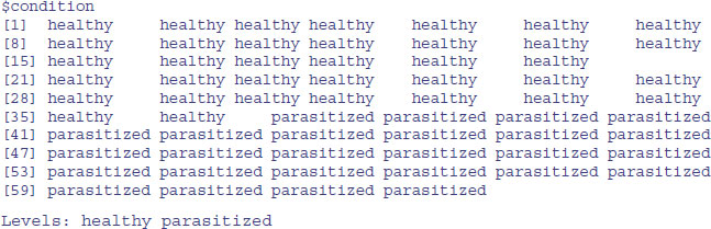
For the purposes of model-fitting, we often want to expand a table of explanatory variables to create a dataframe with as many repeated rows as specified by a count. Here are the data:
count.table<-read.table("c:\\temp\\tabledata.txt",header=T)
attach(count.table)
head(count.table)
count sex age condition
1 12 male young healthy
2 7 male old healthy
3 9 female young healthy
4 8 female old healthy
5 6 male young parasitized
6 7 male old parasitized
The idea is to create a new dataframe with a separate row for each case. That is to say, we want 12 copies of the first row (for healthy young males), seven copies of the second row (for healthy old males), and so on. The trick is to use lapply to apply the repeat function rep to each variable in count.table such that each row is repeated by the number of times specified in the vector called count:

Then we convert this object from a list to a data.frame using as.data.frame like this:
dbtable<-as.data.frame(lapply(count.table,
function(x) rep(x, count.table$count)))
head(dbtable)
count sex age condition
1 12 male young healthy
2 12 male young healthy
3 12 male young healthy
4 12 male young healthy
5 12 male young healthy
6 12 male young healthy
To tidy up, we probably want to remove the redundant vector of counts:
dbtable<-dbtable[,-1]
head(dbtable)
sex age condition
1 male young healthy
2 male young healthy
3 male young healthy
4 male young healthy
5 male young healthy
6 male young healthy
tail(dbtable)
sex age condition
57 female young parasitized
58 female old parasitized
59 female old parasitized
60 female old parasitized
61 female old parasitized
62 female old parasitized
Now we can use the contents of dbtable as explanatory variables in modelling other responses of each of the 62 cases (e.g. the animals' body weights). The alternative is to produce a long vector of row numbers and use this as a subscript on the rows of the short dataframe to turn it into a long dataframe with the same column structure (this is illustrated on p. 255).
6.4 Converting from a dataframe to a table
The reverse procedure of creating a table from a dataframe is much more straightforward, and involves nothing more than the table function:
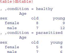
You might want this tabulated object itself to be another dataframe, in which case use:
as.data.frame(table(dbtable))
sex age condition Freq
1 female old healthy 8
2 male old healthy 7
3 female young healthy 9
4 male young healthy 12
5 female old parasitized 5
6 male old parasitized 7
7 female young parasitized 8
8 male young parasitized 6
You will see that R has invented the variable name Freq for the counts of the various contingencies. To change this to ‘count’ use names with the appropriate subscript [4]:
frame<-as.data.frame(table(dbtable))
names(frame)[4]<-"count"
frame
sex age condition count
1 female old healthy 8
2 male old healthy 7
3 female young healthy 9
4 male young healthy 12
5 female old parasitized 5
6 male old parasitized 7
7 female young parasitized 8
8 male young parasitized 6
6.5 Calculating tables of proportions with prop.table
The margins of a table (the row totals or the column totals) are often useful for calculating proportions instead of counts. Here is a data matrix called counts:
counts<-matrix(c(2,2,4,3,1,4,2,0,1,5,3,3),nrow=4)
counts
[,1] [,2] [,3]
[1,] 2 1 1
[2,] 2 4 5
[3,] 4 2 3
[4,] 3 0 3
The proportions will be different when they are expressed as a fraction of the row totals or of the column totals. To find the proportions we use prop.table(counts,margin). You need to remember that the row subscripts come first, which is why margin=1 refers to the row totals:
prop.table(counts,1)
[,1] [,2] [,3]
[1,] 0.5000000 0.2500000 0.2500000
[2,] 0.1818182 0.3636364 0.4545455
[3,] 0.4444444 0.2222222 0.3333333
[4,] 0.5000000 0.0000000 0.5000000
Use margin=2 to express the counts as proportions of the relevant column total:
prop.table(counts,2)
[,1] [,2] [,3]
[1,] 0.1818182 0.1428571 0.08333333
[2,] 0.1818182 0.5714286 0.41666667
[3,] 0.3636364 0.2857143 0.25000000
[4,] 0.2727273 0.0000000 0.25000000
To check that the column proportions sum to 1, use colSums like this:
colSums(prop.table(counts,2))
[1] 1 1 1
If you want the proportions expressed as a fraction of the grand total sum(counts), then simply omit the margin number:
prop.table(counts)
[,1] [,2] [,3]
[1,] 0.06666667 0.03333333 0.03333333
[2,] 0.06666667 0.13333333 0.16666667
[3,] 0.13333333 0.06666667 0.10000000
[4,] 0.10000000 0.00000000 0.10000000
sum(prop.table(counts))
[1] 1
In any particular case, you need to think carefully whether it makes sense to express your counts as proportions of the row totals, the column totals or the grand total.
6.6 The scale function
For a numeric matrix, you might want to scale the values within a column so that they have a mean of 0. You might also want to know the standard deviation of the values within each column. These two actions are carried out simultaneously with the scale function:
scale(counts)
[,1] [,2] [,3]
[1,] -0.7833495 -0.439155 -1.224745
[2,] -0.7833495 1.317465 1.224745
[3,] 1.3055824 0.146385 0.000000
[4,] 0.2611165 -1.024695 0.000000
attr(,"scaled:center")
[1] 2.75 1.75 3.00
attr(,"scaled:scale")
[1] 0.9574271 1.7078251 1.6329932
The values in the table are the counts minus the column means of the counts. The means of the columns attr(,"scaled:center") are 2.75, 1.75 and 3.0, while the standard deviations of the columns attr(,"scaled:scale") are 0.96, 1.71 and 1.63. To check that the scales are the standard deviations (sd) of the counts within a column, you could use apply to the columns (margin = 2) like this:
apply(counts,2,sd)
[1] 0.9574271 1.7078251 1.6329932
6.7 The expand.grid function
This is a useful function for generating tables from factorial combinations of factor levels. Suppose we have three variables: height with five levels between 60 and 80 in steps of 5, weight with five levels between 100 and 300 in steps of 50, and two sexes. Then:
expand.grid(height = seq(60, 80, 5), weight = seq(100, 300, 50),
sex = c("Male","Female"))
height weight sex
1 60 100 Male
2 65 100 Male
3 70 100 Male
4 75 100 Male
5 80 100 Male
…
48 70 300 Female
49 75 300 Female
50 80 300 Female
6.8 The model.matrix function
Creating tables of dummy variables for use in statistical modelling is extremely easy with the model.matrix function. You will see what the function does with a simple example. Suppose that our dataframe contains a factor called parasite indicating the identity of a gut parasite; this variable has five levels: vulgaris, kochii, splendens, viridis and knowlesii. Note that there was no header row in the data file, so the variable name parasite had to be added subsequently, using names:
data<-read.table("c:\\temp\\parasites.txt")
names(data)<-"parasite"
attach(data)
head(data)
parasite
1 vulgaris
2 splendens
3 knowlesii
4 vulgaris
5 knowlesii
6 viridis
levels(parasite)
[1] "knowlesii" "kochii" "splendens" "viridis" "vulgaris"
In our modelling we want to create a two-level dummy variable (present or absent) for each parasite species (in five extra columns), so that we can ask questions such as whether the mean value of the response variable is significantly different in cases where each parasite was present and when it was absent. So for the first row of the dataframe, we want vulgaris = TRUE, knowlesii=FALSE, kochii=FALSE, splendens=FALSE andviridis=FALSE.
The long-winded way of doing this is to create a new factor for each species separately:
vulgaris<-factor(1*(parasite=="vulgaris"))
kochii<-factor(1*(parasite=="kochii"))
table(vulgaris)
vulgaris
0 1
99 52
table(kochii)
kochii
0 1
134 17
and so on, with 1 for TRUE (meaning present) and 0 for FALSE (meaning absent). This is how easy it is to do with model.matrix:

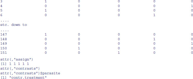
The -1 in the model formula ensures that we create a dummy variable for each of the five parasite species (technically, it suppresses the creation of an intercept). Now we can join these five columns of dummy variables to the dataframe containing the response variable and the other explanatory variables. Suppose we had an original.frame. We just join the new columns to it,
new.frame<-data.frame(original.frame, model.matrix(∼parasite-1))
attach(new.frame)
after which we can use variable names like parasiteknowlesii in statistical modelling.
6.9 Comparing table and tabulate
You will often want to count how many times different values are represented in a vector. This simple example illustrates the difference between the two functions. Here is table in action:
table(c(2,2,2,7,7,11))
2 7 11
3 2 1
It produces names for each element in the vector (2, 7, 11), and counts only those elements that are present (e.g. there are no zeros or ones in the output vector). The tabulate function counts all of the integers (turning real numbers into the nearest integer if necessary), starting at 1 and ending at the maximum (11 in this case), putting a zero in the resulting vector for every missing integer, like this:
tabulate(c(2,2,2,7,7,11))
[1] 0 3 0 0 0 0 2 0 0 0 1
Because there are no 1s in our example, a count of zero is returned for the first element. There are three 2s but then a long gap to two 7s, then another gap to the maximum 11. It is important that you understand that tabulate will ignore negative numbers and zeros without warning:
tabulate(c(2,0,-3,2,2,7,-1, 0,0,7,11))
[1] 0 3 0 0 0 0 2 0 0 0 1
For most applications, table is much more useful than tabulate, but there are occasions when you want the zero counts to be retained. The commonest case is where you are generating a set of vectors, and you want all the vectors to be the same length (e.g. so that you can bind them to a dataframe).
Suppose, for instance, that you want to make a dataframe containing three different realizations of a negative binomial distribution of counts, where the rows contain the frequencies of 0, 1, 2, 3, … successes. Let us take an example where the negative binomial parameters are size = 1 and prob = 0.2 and generate 100 random numbers from it, repeated three times:
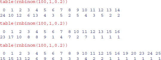
The three realizations produce vectors of different lengths (15, 15 again (but with a 15 and a 16 but no 9 or 14), and 20 respectively). With tabulate, we can specify the length of the output vector (the number of bins, nbins), but we need to make sure it is long enough, because overruns will be ignored without warning. We also need to remember to add 1 to the random integers generated, so that the zeros are counted rather than ignored. From what we have seen (above), it looks as if 30 bins should work well enough, so here are six realizations with nbins=30:

This looks fine, until you check the fifth row. There are only 98 numbers here, so two unknown values of counts greater than 29 have been generated but ignored without warning. To see how often this might happen, we can run the test 1000 times and tally the number of numbers presented by tabulate:
totals<-numeric(1000)
for (i in 1:1000) totals[i] <- sum(tabulate(rnbinom(100,1,0.2)+1,30))
table(totals)
totals
98 99 100
5 114 881
As you see, we lost one or more numbers on 119 occasions out of 1000. So take care with tabulate, and remember that 1 was added to all the counts to accommodate the zeros.