Chapter 12

Analysis of Covariance

Analysis of covariance (ANCOVA) combines elements from regression and analysis of variance. The response variable is continuous, and there is at least one continuous explanatory variable and at least one categorical explanatory variable. The procedure works like this:

• Fit two or more linear regressions of y against x (one for each level of the factor).
• Estimate different slopes and intercepts for each level.
• Use model simplification (deletion tests) to eliminate unnecessary parameters.

For example, we could use ANCOVA in a medical experiment where the response variable was ‘days to recovery’ and the explanatory variables were ‘smoker or not’ (categorical) and ‘blood cell count’ (continuous). In economics, local unemployment rate might be modelled as a function of country (categorical) and local population size (continuous). Suppose we are modelling weight (the response variable) as a function of sex and age. Sex is a factor with two levels (male and female) and age is a continuous variable. The maximal model therefore has four parameters: two slopes (a slope for males and a slope for females) and two intercepts (one for males and one for females) like this:

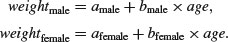
This maximal model is shown in the top left-hand panel. Model simplification is an essential part of analysis of covariance, because the principle of parsimony requires that we keep as few parameters in the model as possible.

There are six possible models in this case, and the process of model simplification begins by asking whether we need all four parameters (top left). Perhaps we could make do with two intercepts and a common slope (top right), or a common intercept and two different slopes (centre left). There again, age may have no significant effect on the response, so we only need two parameters to describe the main effects of sex on weight; this would show up as two separated, horizontal lines in the plot (one mean weight for each sex; centre right). Alternatively, there may be no effect of sex at all, in which case we only need two parameters (one slope and one intercept) to describe the effect of age on weight (bottom left). In the limit, neither the continuous nor the categorical explanatory variables might have any significant effect on the response, in which case model simplification will lead to the one-parameter null model (a single horizontal line; bottom right).

12.1 Analysis of covariance in R

We could use either lm or aov; the choice affects only the format of the summary table. We shall use both and compare their output. Our worked example concerns an experiment on the impact of grazing on the seed production of a biennial plant. Forty plants were allocated to two treatments, grazed and ungrazed, and the grazed plants were exposed to rabbits during the first two weeks of stem elongation. They were then protected from subsequent grazing by the erection of a fence and allowed to regrow. Because initial plant size was thought likely to influence fruit production, the diameter of the top of the rootstock was measured before each plant was potted up. At the end of the growing season, the fruit production (dry weight in milligrams) was recorded on each of the 40 plants, and this forms the response variable in the following analysis.

regrowth <- read.table("c:\\temp\\ipomopsis.txt",header=T)

attach(regrowth)

names(regrowth)

[1] "Root" "Fruit" "Grazing"

The object of the exercise is to estimate the parameters of the minimal adequate model for these data. We begin by inspecting the data with a plot of fruit production against root size for each of the two treatments separately:

plot(Root,Fruit,pch=16,col=c("blue","red")[as.numeric(Grazing)])

where red dots represent the ungrazed plants and blue dots represent the grazed plants. Note the use of as.numeric to select the plotting colours. How are the grazing treatments reflected in the factor levels?

levels(Grazing)

[1] "Grazed" "Ungrazed"

Now we can use logical subscripts (p. 39) to draw linear regression lines for the two grazing treatments separately, using abline (we could have used subset instead):

abline(lm(Fruit[Grazing=="Grazed"]∼Root[Grazing=="Grazed"]),col="blue")

abline(lm(Fruit[Grazing=="Ungrazed"]∼Root[Grazing=="Ungrazed"]),col="red")

The odd thing about these data is that grazing seems to increase fruit production, which is a highly counter-intuitive result:

tapply(Fruit,Grazing, mean)

Grazed	Ungrazed

67.9405	50.8805

This difference is statistically significant (p = 0.027) if you do a t test (although this is the wrong thing to do in this case, as explained below):

t.test(Fruit∼Grazing)

	Welch Two Sample t-test

data: Fruit by Grazing

t = 2.304, df = 37.306, p-value = 0.02689

alternative hypothesis: true difference in means is not equal to 0

95 percent confidence interval:

2.061464 32.058536

sample estimates:

mean in group Grazed mean in group Ungrazed

	67.9405		50.8805

Several important points are immediately apparent from this initial analysis:

• Different sized plants were allocated to the two treatments.
• The grazed plants were bigger at the outset.
• The regression line for the ungrazed plants is above the line for the grazed plants.
• The regression lines are roughly parallel.
• The intercepts (not shown to the left) are likely to be significantly different.

Each of these points will be addressed in detail.

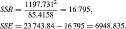
To understand the output from analysis of covariance it is useful to work through the calculations by hand. We start by working out the sums, sums of squares and sums of products for the whole data set combined (40 pairs of numbers), and then for each treatment separately (20 pairs of numbers). We shall fill in a table of totals, because it helps to be really well organized for these calculations. Check to see where (and why) the sums and the sums of squares of the root diameters (the x values) and the fruit yields (the y values) have gone in the table. First, we shall work out the overall totals based on all 40 data points.

sum(Root);sum(Root^2)

[1] 287.246

[1] 2148.172

sum(Fruit);sum(Fruit^2)

[1] 2376.42

[1] 164928.1

sum(Root*Fruit)

[1] 18263.16

These are the famous five, which we shall make use of shortly, and complete the overall data summary. Now we select the root diameters for the grazed and ungrazed plants and then the fruit yields for the grazed and ungrazed plants:

sum(Root[Grazing=="Grazed"]);sum(Root[Grazing=="Grazed"]^2)

[1] 166.188

[1] 1400.834

sum(Root[Grazing=="Ungrazed"]);sum(Root[Grazing=="Ungrazed"]^2)

[1] 121.058

[1] 747.3387

sum(Fruit[Grazing=="Grazed"]);sum(Fruit[Grazing=="Grazed"]^2)

[1] 1358.81

[1] 104156.0

sum(Fruit[Grazing=="Ungrazed"]);sum(Fruit[Grazing=="Ungrazed"]^2)

[1] 1017.61

[1] 60772.11

Finally, we want the sums of products: first for the grazed plants and then for the ungrazed plants:

sum(Root[Grazing=="Grazed"]*Fruit[Grazing=="Grazed"])

[1] 11753.64

sum(Root[Grazing=="Ungrazed"]*Fruit[Grazing=="Ungrazed"])

[1] 6509.522

Here is our table:

	Sums	Squares and products
x ungrazed	121.058	747.3387
y ungrazed	1017.61	60772.11
xy ungrazed		6509.522
x grazed	166.188	1400.834
y grazed	1358.81	104156.0
xy grazed		11753.64
x overall	287.246	2148.172
y overall	2376.42	164928.1
xy overall		18263.16

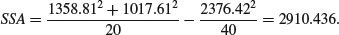
Now we have all of the information necessary to carry out the calculations of the corrected sums of squares and products, SSY, SSX and SSXY, for the whole data set (n = 40) and for the two separate treatments (with 20 replicates in each). To get the right answer you will need to be extremely methodical, but there is nothing mysterious or difficult about the process. First, calculate the regression statistics for the whole experiment, ignoring the grazing treatment, using the famous five which we have just calculated:

The effect of differences between the two grazing treatments, SSA, is

Next calculate the regression statistics for each of the grazing treatments separately. First, for the grazed plants:

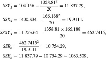
so the slope of the graph of Fruit against Root for the grazed plants is given by

Now for the ungrazed plants:

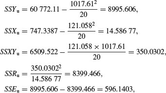
so the slope of the graph of Fruit against Root for the ungrazed plants is given by

Now add up the regression statistics across the factor levels (grazed and ungrazed):

The SSR for a model with a single common slope is given by

and the value of the single common slope is

The difference between the two estimates of SSR (SSRdiff = SSRg+u – SSRc = 19 153.75 – 19 148.94 = 4.81) is a measure of the significance of the difference between the two slopes estimated separately for each factor level. Finally, SSE is calculated by difference:

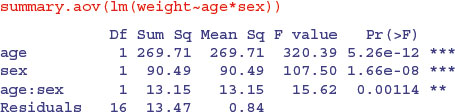
Now we can complete the ANOVA table for the full model:

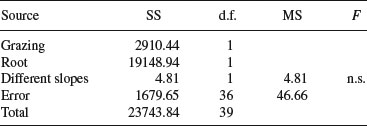
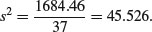
Degrees of freedom for error are 40 – 4 = 36 because we have estimated four parameters from the data: two slopes and two intercepts. So the error variance is 46.66 (= SSE/36). The difference between the slopes is clearly not significant (F = 4.81/46.66 = 0.10) so we can fit a simpler model with a common slope of 23.56. The sum of squares for differences between the slopes (4.81) now becomes part of the error sum of squares:

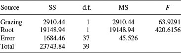
This is the minimal adequate model. Both of the terms are highly significant and there are no redundant factor levels.

The next step is to calculate the intercepts for the two parallel regression lines. This is done exactly as before, by rearranging the equation of the straight line to obtain a = y – bx. For each line we can use the mean values of x and y, with the common slope in each case. Thus:

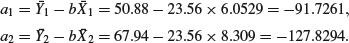
This demonstrates that the grazed plants produce, on average, 127.83 – 91.73 = 36.1 mg of fruit less than the ungrazed plants.

Finally, we need to calculate the standard errors for the common regression slope and for the difference in mean fecundity between the treatments, based on the error variance in the minimal adequate model, given in the table above:

The standard errors are obtained as follows. The standard error of the common slope is found in the usual way:

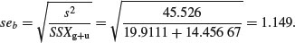
The standard error of the intercept of the regression for the grazed treatment is also found in the usual way:

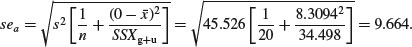
It is clear that the intercept of –127.829 is very significantly less than zero (t = 127.829/9.664 = 13.2), suggesting that there is a threshold rootstock size before reproduction can begin. The standard error of the difference between the elevations of the two lines (the grazing effect) is given by

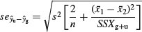
which, substituting the values for the error variance and the mean rootstock sizes of the plants in the two treatments, becomes:

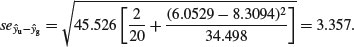
This suggests that any lines differing in elevation by more than about 2 × 3.357 = 6.71 mg dry weight would be regarded as significantly different. Thus, the present difference of 36.09 clearly represents a highly significant reduction in fecundity caused by grazing (t = 10.83).

The hand calculations were convoluted, but ANCOVA is exceptionally straightforward in R, using lm. The response variable is fecundity (Fruit), and there is one experimental factor (Grazing) with two levels (Ungrazed and Grazed) and one covariate (initial rootstock diameter, Root). There are 40 values for each of these variables. As we saw earlier, the largest plants were allocated to the grazed treatments, but for a given rootstock diameter (say, 7 mm) the scatterplot shows that the grazed plants produced fewer fruits than the ungrazed plants (not more, as a simple comparison of the means suggested). This is an excellent example of the value of analysis of covariance. Here, the correct analysis using ANCOVA completely reverses our interpretation of the data.

The analysis proceeds in the following way. We fit the most complicated model first, then simplify it by removing non-significant terms until we are left with a minimal adequate model, in which all the parameters are significantly different from zero. For ANCOVA, the most complicated model has different slopes and intercepts for each level of the factor. Here we have a two-level factor (Grazed and Ungrazed) and we are fitting a linear model with two parameters (y = a + bx) so the most complicated mode has four parameters (two slopes and two intercepts). To fit different slopes and intercepts we use the asterisk * notation:

ancova <- lm(Fruit∼Grazing*Root)

You should realize that order matters: we would get a different output if the model had been written Fruit ∼ Root * Grazing (more of this on p. 555).

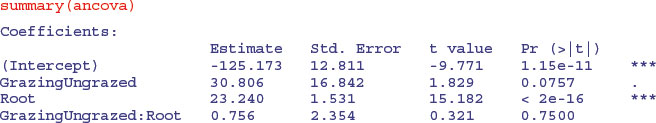
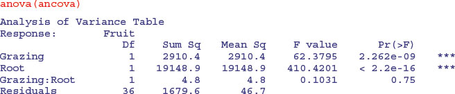
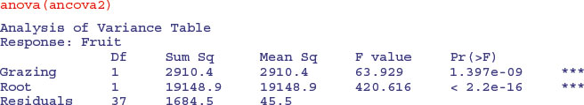
This shows that initial root size has a massive effect on fruit production (t = 15.182), but there is no indication of any difference in the slope of this relationship between the two grazing treatments (this is the Grazing by Root interaction with t = 0.321, ). The ANOVA table for the maximal model looks like this:

The next step is to delete the non-significant interaction term from the model. We can do this manually or automatically: here we shall do both for the purposes of demonstration. The function for manual model simplification is update. We update the current model (here called ancova) by deleting terms from it. The syntax is important: the punctuation reads ‘comma tilde dot minus’. We define a new name for the simplified model:

ancova2 <- update(ancova, ∼ . - Grazing:Root)

Now we compare the simplified model with just three parameters (one slope and two intercepts) with the maximal model using anova like this:

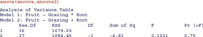
This says that model simplification was justified because it caused a negligible reduction in the explanatory power of the model (p = 0.75; to retain the interaction term in the model we would need p < 0.05).

The next step in model simplification involves testing whether or not grazing had a significant effect on fruit production once we control for initial root size. The procedure is similar: we define a new model and use update to remove Grazing from ancova2 like this:

ancova3 <- update(ancova2, ∼ . - Grazing)

Now we compare the two models using anova:

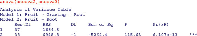
This model simplification is a step too far. Removing the Grazing term causes a massive reduction in the explanatory power of the model, with an F value of 115.63 and a vanishingly small p value. The effect of grazing in reducing fruit production is highly significant and needs to be retained in the model. Thus ancova2 is our minimal adequate model, and we should look at its summary table to compare with our earlier calculations carried out by hand:

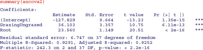
You know when you have got the minimal adequate model, because every row of the coefficients table has one or more significance stars (three in this case, because the effects are all so strong). In contrast to our initial interpretation based on mean fruit production, grazing is associated with a 36.103 mg reduction in fruit production.

These are the values we obtained the long way on p. 540.

Now we repeat the model simplification using the automatic model-simplification function called step. It could not be easier to use. The full model is called ancova:

step(ancova)

This function causes all the terms to be tested to see whether they are needed in the minimal adequate model. The criterion used is Akaike's information criterion (AIC, p. 415). In the jargon, this is a ‘penalized log-likelihood’. What this means in simple terms is that it weighs up the inevitable trade-off between degrees of freedom and fit of the model. You can have a perfect fit if you have a parameter for every data point, but this model has zero explanatory power. Thus deviance goes down as degrees of freedom in the model go up. The AIC adds 2 times the number of parameters in the model to the deviance (to penalize it). Deviance, you will recall, is twice the log-likelihood of the current model. Anyway, AIC is a measure of lack of fit; big AIC is bad, small AIC is good. The full model (four parameters: two slopes and two intercepts) is fitted first, and AIC calculated as 157.5:

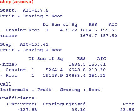
Then step tries removing the most complicated term (the Grazing by Root interaction). This reduces AIC to 155.61 (an improvement, so the simplification is justified). No further simplification is possible (as we saw when we used update to remove the Grazing term from the model) because AIC goes up to 210.3 when Grazing is removed and up to 254.2 if Root is removed. Thus, step has found the minimal adequate model (it does not always do so, as we shall see later; it is good, but not perfect).

12.2 ANCOVA and experimental design

There is an extremely important general message in this example for experimental design. No matter how carefully we randomize at the outset, our experimental groups are likely to be heterogeneous. Sometimes, as in this case, we may have made initial measurements that we can use as covariates later on, but this will not always be the case. There are bound to be important factors that we did not measure. If we had not measured initial root size in this example, we would have come to entirely the wrong conclusion about the impact of grazing on plant performance.

A far better design for this experiment would have been to measure the rootstock diameters of all the plants at the beginning of the experiment (as was done here), but then to place the plants in matched pairs with rootstocks of similar size. Then, one of the plants would be picked at random and allocated to one of the two grazing treatments (e.g. by tossing a coin); the other plant of the pair then receives the unallocated gazing treatment. Under this scheme, the size ranges of the two treatments would overlap, and the analysis of covariance would be unnecessary.

12.3 ANCOVA with two factors and one continuous covariate

The following experiment, with weight as the response variable, involved genotype and sex as two categorical explanatory variables and age as a continuous covariate. There are six levels of genotype and two levels of sex.

Gain <- read.table("c:\\temp\\Gain.txt",header=T)

attach(Gain)

names(Gain)

[1] "Weight" "Sex" "Age" "Genotype" "Score"

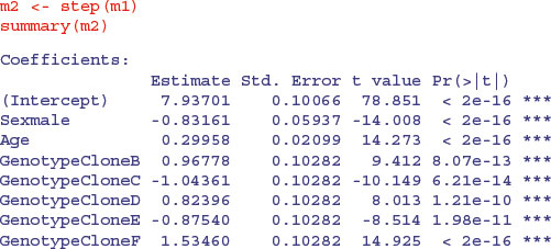
We begin by fitting the maximal model with its 24 parameters: there are different slopes and intercepts for every combination of sex and genotype (2 × 6 × 2 = 24).

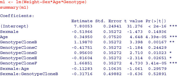
You should work through this output slowly and make sure that you can see what each term means. Remember that the intercept is for all the factor levels that come first in the alphabet (females of CloneA) and the slope (Age) likewise. There is only one intercept and one slope in this entire output. Everything else is either a difference between intercepts, or a difference between slopes. Names involving Age are differences between slopes; names not involving Age are differences between intercepts.

There are one or two significant parameters, but it is not at all clear that the three-way or two-way interactions need to be retained in the model. As a first pass, let us use step to see how far it gets with model simplification:

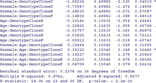
We definitely do not need the three-way interaction, despite the effect of Sexmale:Age: GenotypeCloneC which gave a significant t test on its own. How about the three two-way interactions? The step function leaves out Sex by Genotype and then assesses the other two. No need for Age by Genotype. Try removing Sex by Age. Nothing. What about the main effects? They are all highly significant. This is R's idea of the minimal adequate model: three main effects but no interactions. That is to say, the slope of the graph of weight gain against age does not vary with sex or genotype, but the intercepts do vary.

This is where Helmert contrasts would actually come in handy (see p. 553). Everything is three-star significantly different from Genotype[1] Sex[1], but it is not obvious that the intercepts for genotypes B and D need different values (+0.96 and +0.82 above genotype A with sediff = 0.1028), nor is it obvious that C and E have different intercepts (–1.043 and –0.875). Perhaps we could reduce the number of factor levels of Genotype from the present six to four without any loss of explanatory power ?

We create a new categorical variable called newGenotype with separate levels for clones A and F, and for B and D combined and C and E combined:

newGenotype <- Genotype

levels(newGenotype)

[1] "CloneA" "CloneB" "CloneC" "CloneD" "CloneE" "CloneF"

levels(newGenotype)[c(3,5)] <- "ClonesCandE"

levels(newGenotype)[c(2,4)] <- "ClonesBandD"

levels(newGenotype)

[1] "CloneA" "ClonesBandD" "ClonesCandE" "CloneF"

Then we redo the modelling with newGenotype (four levels) instead of Genotype (six levels),

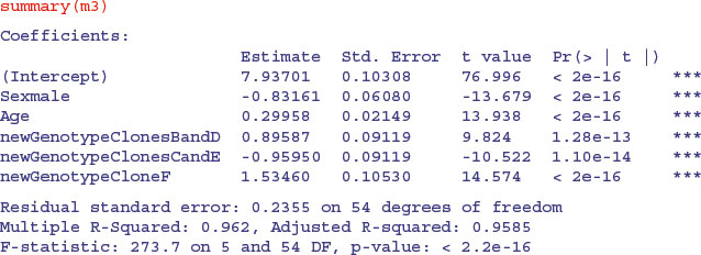
m3 <- lm(Weight∼Sex+Age+newGenotype)

and check that the simplification was justified:

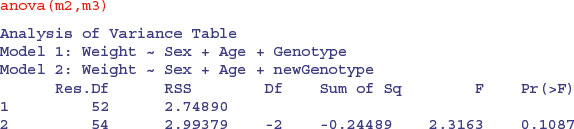
Yes, the simplification was justified (p value = 0.1087) so we accept the simpler model m3:

After an analysis of covariance, it is useful to draw the fitted lines through a scatterplot, with each factor level represented by different plotting symbols and line types (see p. 198):

plot(Age,Weight,type="n")

colours <- c("green","red","black","blue")

lines <- c(1,2)

symbols <- c(16,17)

points(Age,Weight,pch=symbols[as.numeric(Sex)],

	col=colours[as.numeric(newGenotype)])

xv <- c(1,5)

for (i in 1:2) {

for (j in 1:4) {

	a <- coef(m3)[1]+(i>1)* coef(m3)[2]+(j>1)*coef(m3)[j+2]

	b <- coef(m3)[3]

	yv <- a+b*xv

lines(xv,yv,lty=lines[i],col=colours[j]) } }

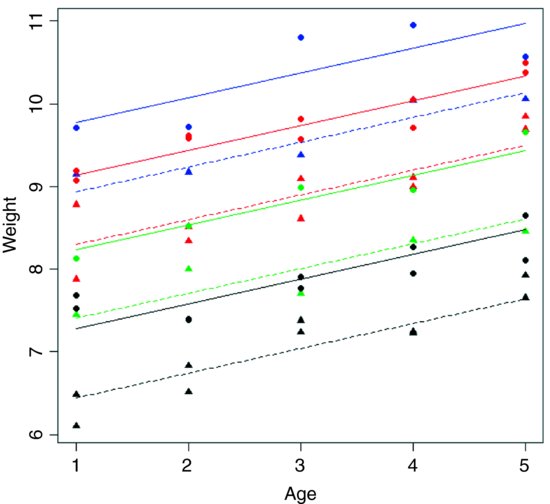
Note the use of colour to represent the four genotypes and plotting symbols and line types to represent the two sexes. You can see that the males (circles and solid lines) are heavier than the females (triangles and dashed lines) in all of the genotypes. Other functions to be considered in plotting the results of ANCOVA are split and augPred in lattice graphics.

12.4 Contrasts and the parameters of ANCOVA models

In analysis of covariance, we estimate a slope and an intercept for each level of one or more factors. Suppose we are modelling weight (the response variable) as a function of sex and age, as illustrated on p. 538. The difficulty arises because there are several different ways of expressing the values of the four parameters in the summary.lm table:

• two slopes, and two intercepts (as in the equations on p. 537);
• one slope and one difference between slopes, and one intercept and one difference between intercepts;
• the overall mean slope and the overall mean intercept, and one difference between slopes and one difference between intercepts.

In the second case (two estimates and two differences) a decision needs to be made about which factor level to associate with the estimate, and which level with the difference (e.g. whether males should be expressed as the intercept and females as the difference between intercepts, or vice versa) .

When the factor levels are unordered (the typical case), then R takes the factor level that comes first in the alphabet as the estimate and the others are expressed as differences. In our example, the parameter estimates would be female, and male parameters would be expressed as differences from the female values, because ‘f’ comes before ‘m’ in the alphabet. This should become clear from an example:

Ancovacontrasts <- read.table("c:\\temp\\Ancovacontrasts.txt",header=T)

attach(Ancovacontrasts)

names(Ancovacontrasts)

[1] "weight" "sex" "age"

First we work out the two regressions separately so that we know the values of the two slopes and the two intercepts (note the use of subscripts or subsets to select the sexes):

lm(weight[sex=="male"]∼age[sex=="male"])

Coefficients:

 (Intercept) age[sex == "male"]

	3.115		1.561

lm(weight∼age,subset=(sex=="female"))

Coefficients:

	(Intercept)	age

	1.9663		0.9962

So the intercept for males is 3.115 and the intercept for females is 1.9663. The difference between the first (female) and second (male) intercepts is therefore

and the difference between the two slopes is

Now we can do an overall regression, ignoring gender:

lm(weight∼age)

Call:

lm(formula = weight ∼ age)

Coefficients:

(Intercept)		age

 2.541			1.279

This tells us that the average intercept is 2.541 and the average slope is 1.279.

Next we can carry out an analysis of covariance and compare the output produced by each of the three different contrast options allowed by R: treatment (the default in R and Glim), Helmert (the default in S-PLUS), and sum. First, the analysis using treatment contrasts as used by R and Glim:

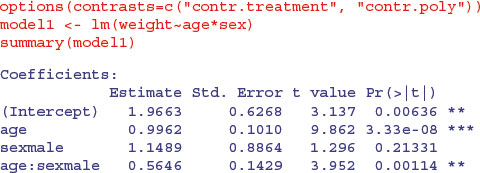
The intercept (1.9663) is the intercept for females (because ‘f’ comes before ‘m’ in the alphabet). The age parameter (0.9962) is the slope of the graph of weight against age for females. The sex parameter (1.1489) is the difference between the (female) intercept and the male intercept (1.9663 + 1.1489 = 3.1152). The age–sex interaction term is the difference between slopes of the female and male graphs (0.9962 + 0.5646 = 1.5608). So with treatment contrasts, the parameters (in order 1 to 4) are an intercept, a slope, a difference between two intercepts, and a difference between two slopes. In the standard error column we see, from row 1 downwards, the standard error of an intercept for a regression with females only (0.6268 with n = 10, Σ x2 = 385 and SSX = 82.5), the standard error of a slope for females only (0.1010, with SSX = 82.5), the standard error of the difference between two intercepts each based on n = 10 data points 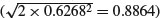and the standard error of the difference between two slopes each based on n = 10 data points 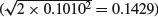. The formulas for these standard errors are on p. 554. Many people are more comfortable with this method of presentation than they are with Helmert or sum contrasts.

We now turn to the analysis using Helmert contrasts:

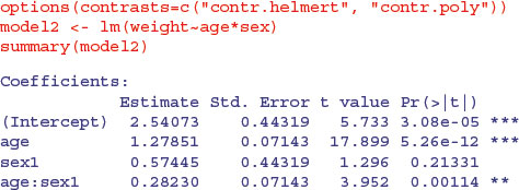
Let us see if we can work out what the four parameter values represent. The first parameter, 2.540 73 (labelled Intercept), is the intercept of the overall regression, ignoring sex (see above). The parameter labelled age (1.278 51) is a slope because age is our continuous explanatory variable. Again, you will see that it is the slope for the regression of weight against age, ignoring sex. The third parameter, labelled sex1 (0.574 45), must have something to do with intercepts because sex is our categorical variable. If we want to reconstruct the second intercept (for males) we need to add 0.574 45 to the overall intercept: 2.540 73 + 0.574 45 = 3.115 18. To get the intercept for females we need to subtract it: 2.540 73 – 0.574 45 = 1.966 28. The fourth parameter (0.282 30), labelled age:sex1, is the difference between the overall mean slope (1.278 51) and the male slope: 1.278 51 + 0.282 30 = 1.560 81. To get the slope of weight against age for females we need to subtract the interaction term from the age term: 1.278 51 – 0.282 30 = 0.996 21.

In the standard errors column, from the top row downwards, you see the standard error of an intercept based on a regression with all 20 points (the overall regression, ignoring sex, 0.443 19) and the standard error of a slope based on a regression with all 20 points (0.071 43). The standard errors of differences (both intercept and slope) involve half the difference between the male and female values, because with Helmert contrasts the difference is between the male value and the overall value, rather than between the male and female values. Thus the third row has the standard error of a difference between the overall intercept and the intercept for males based on a regression with 10 points (0.443 19 = 0.8864/2), and the bottom row has the standard error of a difference between the overall slope and the slope for males, based on a regression with 10 points (0.1429/2 = 0.071 43). Thus the values in the bottom two rows of the Helmert table are simply half the values in the same rows of the treatment table.

The advantage of Helmert contrasts is in hypothesis testing in more complicated models than this, because it is easy to see which terms we need to retain in a simplified model by inspecting their significance levels in the summary.lm table. The disadvantage is that it is much harder to reconstruct the slopes and the intercepts from the estimated parameters values (see also p. 440).

Finally, we look at the third option, which is sum contrasts:

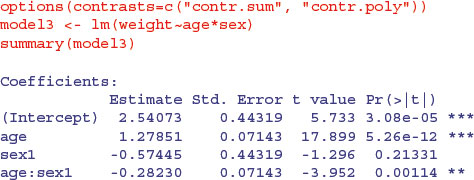
The first two estimates are the same as those produced by Helmert contrasts: the overall intercept and slope of the graph relating weight to age, ignoring sex. The sex parameter (–0.574 45) is sign reversed compared with the Helmert option: it shows how to calculate the female (the first) intercept from the overall intercept 2.540 73– 0.574 45 = 1.966 28. The interaction term also has reversed sign: to get the slope for females, add the interaction term to the slope for age: 1.278 51– 0.282 30 = 0.996 21.

The four standard errors for the sum contrasts are exactly the same as those for Helmert contrasts (explained above).

12.5 Order matters in summary.aov

People are often disconcerted by the ANOVA table produced by summary.aov in analysis of covariance. Compare the tables produced for these two models:

Exactly the same sums of squares and p values. No problem. But look at these two models from the plant compensation example analysed in detail earlier (p. 545):

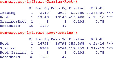
In this case the order of variables within the model formula has a huge effect: it changes the sum of squares associated with the two main effects (root size is continuous and grazing is categorical, grazed or ungrazed) and alters their p values. The interaction term, the residual sum of squares and the error variance are unchanged. So what is the difference between the two cases?

In the first example, where order was irrelevant, the x values for the continuous variable (age) were identical for both sexes (there is one male and one female value at each of the 10 experimentally controlled ages). In the second example, the x values (root size) were different in the two treatments, and mean root size was greater for the grazed plants than for the ungrazed ones:

tapply(Root,Grazing, mean)

Grazed Ungrazed

8.3094	6.0529

Whenever the x values are different in different factor levels, and/or there is different replication in different factor levels, then SSX and SSXY will vary from level to level and this will affect the way the sum of squares is distributed across the main effects. It is of no consequence in terms of your interpretation of the model, however, because the effect sizes and standard errors in the summary.lm table are completely unaffected:

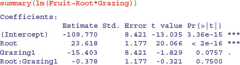
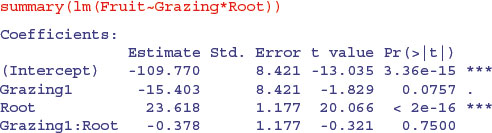
The p values that are shown in summary.lm are the deletion p values that we are accustomed to. The p values in the full ANOVA table, however, are not. Once the interaction term is deleted, the problem disappears, and the p values, once again, are the familiar deletion p values.