Chapter 13

Generalized Linear Models

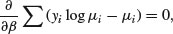
We can use generalized linear models (GLMs) – pronounced ‘glims’ – when the variance is not constant, and/or when the errors are not normally distributed. Certain kinds of response variables invariably suffer from these two important contraventions of the standard assumptions, and GLMs are excellent at dealing with them. Specifically, we might consider using GLMs when the response variable is:

• count data expressed as proportions (e.g. logistic regressions);
• count data that are not proportions (e.g. log-linear models of counts);
• binary response variables (e.g. dead or alive);
• data on time to death where the variance increases faster than linearly with the mean (e.g. time data with gamma errors).

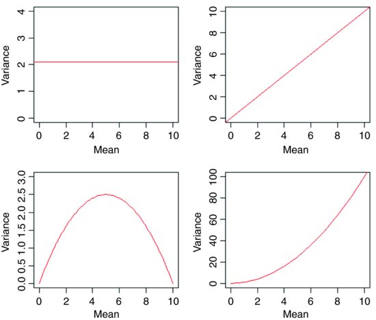
The central assumption that we have made up to this point is that variance was constant (top left-hand graph). In count data, however, where the response variable is an integer and there are often lots of zeros in the dataframe, the variance may increase linearly with the mean (top tight). With proportion data, where we have a count of the number of failures of an event as well as the number of successes, the variance will be an inverted U-shaped function of the mean (bottom left). Where the response variable follows a gamma distribution (as in time-to-death data) the variance increases faster than linearly with the mean (bottom right). Many of the basic statistical methods such as regression and Student's t test assume that variance is constant, but in many applications this assumption is untenable. Hence the great utility of GLMs.

A GLM has three important properties:

• the error structure;
• the linear predictor;
• the link function.

These are all likely to be unfamiliar concepts. The ideas behind them are straightforward, however, and it is worth learning what each of the concepts involves.

13.1 Error structure

Up to this point, we have dealt with the statistical analysis of data with normal errors. In practice, however, many kinds of data have non-normal errors: for example:

• errors that are strongly skewed;
• errors that are kurtotic;
• errors that are strictly bounded (as in proportions);
• errors that cannot lead to negative fitted values (as in counts).

In the past, the only tools available to deal with these problems were transformation of the response variable or the adoption of non-parametric methods. A GLM allows the specification of a variety of different error distributions:

• Poisson errors, useful with count data;
• binomial errors, useful with data on proportions;
• gamma errors, useful with data showing a constant coefficient of variation;
• exponential errors, useful with data on time to death (survival analysis).

The error structure is defined by means of the family directive, used as part of the model formula. Examples are

glm(y ∼ z, family = poisson)

which means that the response variable y has Poisson errors, and

glm(y ∼ z, family = binomial)

which means that the response is binary, and the model has binomial errors. As with previous models, the explanatory variable z can be continuous (leading to a regression analysis) or categorical (leading to an ANOVA-like procedure called analysis of deviance, as described below).

13.2 Linear predictor

The structure of the model relates each observed y value to a predicted value. The predicted value is obtained by transformation of the value emerging from the linear predictor. The linear predictor, η (eta), is a linear sum of the effects of one or more explanatory variables, xj,

where the xs are the values of the p different explanatory variables, and the βs are the (usually) unknown parameters to be estimated from the data. The right-hand side of the equation is called the linear structure.

There are as many terms in the linear predictor as there are parameters, p, to be estimated from the data. Thus, with a simple regression, the linear predictor is the sum of two terms whose parameters are the intercept and the slope. With a one-way ANOVA with four treatments, the linear predictor is the sum of four terms leading to the estimation of the mean for each level of the factor. If there are covariates in the model, they add one term each to the linear predictor (the slope of each relationship). Interaction terms in a factorial ANOVA add one or more parameters to the linear predictor, depending upon the degrees of freedom of each factor (e.g. there would be three extra parameters for the interaction between a two-level factor and a four-level factor, because (2 – 1) × (4 – 1) = 3).

To determine the fit of a given model, a GLM evaluates the linear predictor for each value of the response variable, then compares the predicted value with a transformed value of y. The transformation to be employed is specified in the link function, as explained below. The fitted value is computed by applying the reciprocal of the link function, in order to get back to the original scale of measurement of the response variable.

13.3 Link function

One of the difficult things to grasp about GLMs is the relationship between the values of the response variable (as measured in the data and predicted by the model in fitted values) and the linear predictor. The thing to remember is that the link function relates the mean value of y to its linear predictor. In symbols, this means that

which is simple, but needs thinking about. The linear predictor, η, emerges from the linear model as a sum of the terms for each of the p parameters. This is not a value of y (except in the special case of the identity link that we have been using (implicitly) up to now). The value of η is obtained by transforming the value of y by the link function, and the predicted value of y is obtained by applying the inverse link function to η.

The most frequently used link functions are shown below. An important criterion in the choice of link function is to ensure that the fitted values stay within reasonable bounds. We would want to ensure, for example, that counts were all greater than or equal to 0 (negative count data would be nonsense). Similarly, if the response variable was the proportion of individuals that died, then the fitted values would have to lie between 0 and 1 (fitted values greater than 1 or less than 0 would be meaningless). In the first case, a log link is appropriate because the fitted values are antilogs of the linear predictor, and all antilogs are greater than or equal to 0. In the second case, the logit link is appropriate because the fitted values are calculated as the antilogs of the log odds, log(p/q).

By using different link functions, the performance of a variety of models can be compared directly. The total deviance is the same in each case, and we can investigate the consequences of altering our assumptions about precisely how a given change in the linear predictor brings about a response in the fitted value of y. The most appropriate link function is the one which produces the minimum residual deviance.

13.3.1 Canonical link functions

The canonical link functions are the default options employed when a particular error structure is specified in the family directive in the model formula. Omission of a link directive means that the following settings are used:

Error	Canonical link
normal	identity
poisson	log
binomial	logit
Gamma	reciprocal

You should try to memorize these canonical links and to understand why each is appropriate to its associated error distribution. Note that only gamma errors have a capital initial letter in R.

Choosing between using a link function (e.g. log link) and transforming the response variable (i.e. having log(y) as the response variable rather than y) takes a certain amount of experience. The decision is usually based on whether the variance is constant on the original scale of measurement. If the variance was constant, you would use a link function. If the variance increased with the mean, you would be more likely to log-transform the response.

13.4 Proportion data and binomial errors

Proportion data have three important properties that affect the way the data should be analysed:

• the data are strictly bounded;
• the variance is non-constant;
• errors are non-normal.

You cannot have a proportion greater than 1 or less than 0. This has obvious implications for the kinds of functions fitted and for the distributions of residuals around these fitted functions. For example, it makes no sense to have a linear model with a negative slope for proportion data because there would come a point, with high levels of the x variable, where negative proportions would be predicted. Likewise, it makes no sense to have a linear model with a positive slope for proportion data because there would come a point, with high levels of the x variable, where proportions greater than 1 would be predicted.

With proportion data, if the probability of success is 0, then there will be no successes in repeated trials, all the data will be zeros and hence the variance will be zero. Likewise, if the probability of success is 1, then there will be as many successes as there are trials, and again the variance will be 0. For proportion data, therefore, the variance increases with the mean up to a maximum (when the probability of success is 0.5) then declines again towards zero as the mean approaches 1. The variance–mean relationship is humped, rather than constant as assumed in the classical tests.

The final assumption is that the errors (the differences between the data and the fitted values estimated by the model) are normally distributed. This cannot be so in proportional data because the data are bounded above and below: no matter how big a negative residual might be at high predicted values, a positive residual cannot be bigger than . Similarly, no matter how big a positive residual might be for low predicted values , a negative residual cannot be greater than (because you cannot have negative proportions). This means that confidence intervals must be asymmetric whenever takes large values (close to 1) or small values (close to 0).

All these issues (boundedness, non-constant variance, non-normal errors) are dealt with by using a generalized linear model with a binomial error structure. It could not be simpler to deal with this. Instead of using a linear model and writing

lm(y∼x)

we use a generalized linear model and specify that the error family is binomial like this:

glm(y∼x,family=binomial)

That's all there is to it. In fact, it is even easier than that, because we do not even need to write family=:

glm(y∼x,binomial)

13.5 Count data and Poisson errors

Count data have a number of properties that need to be considered during modelling:

• Count data are bounded below (you cannot have counts less than zero).
• Variance is not constant (variance increases with the mean).
• Errors are not normally distributed.
• The fact that the data are whole numbers (integers) affects the error distribution.

It is very simple to deal with all these issues by using a GLM. All we need to write is

glm(y∼x,poisson)

and the model is fitted with a log link (to ensure that the fitted values are bounded below) and Poisson errors (to account for the non-normality). If, having fitted the minimal adequate model, we discover that the residual deviance is greater than the residual degrees of freedom, then we have contravened an important assumption of the model. This is called overdispersion, and we can correct for it by specifying quasipoisson errors like this:

glm(y∼x,quasipoisson)

It is important to understand that Poisson errors are an assumption, not a fact. Many of the count data you encounter in practice will have variance–mean ratios greater than 1, and in these cases you will need to correct for overdispersion.

13.6 Deviance: Measuring the goodness of fit of a GLM

The fitted values produced by the model are most unlikely to match the values of the data perfectly. The size of the discrepancy between the model and the data is a measure of the inadequacy of the model; a small discrepancy may be tolerable, but a large one will not be. The measure of discrepancy in a GLM to assess the goodness of fit of the model to the data is called the deviance. Deviance is defined as –2 times the difference in log-likelihood between the current model and a saturated model (i.e. a model that fits the data perfectly). Because the latter does not depend on the parameters of the model, minimizing the deviance is the same as maximizing the likelihood.

Deviance is estimated in different ways for different families within glm (Table 13.1). Numerical examples of the calculation of deviance for different glm families are given in Chapters 14 (Poisson errors), 16 (binomial errors), and 27 (gamma errors). Where there is grouping structure in the data, leading to spatial or temporal pseudoreplication, you will want to use generalized mixed models (lmer) with one of these error families (p. 710).

Table 13.1 Deviance formulae for different GLM families, where y is observed data, the mean value of y, μ are the fitted values of y from the maximum likelihood model, and n is the binomial denominator in a binomial GLM.

Family (error structure)	Deviance	Variance function
gaussian		1
poisson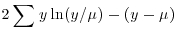
binomial
Gamma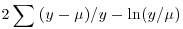
inverse.gaussian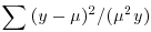

13.7 Quasi-likelihood

The precise relationship between the variance and the mean is well established for all the GLM error families (Table 13.1). In some cases, however, we may be uneasy about specifying the precise form of the error distribution. We may know, for example, that it is not normal (e.g. because the variance increases with the mean), but we do not know with any confidence that the underlying distribution is, say, negative binomial.

There is a very simple and robust alternative known as quasi-likelihood, introduced by Wedderburn (1974), which uses only the most elementary information about the response variable, namely the variance–mean relationship (see Taylor's power law, p. 262). It is extraordinary that this information alone is often sufficient to retain close to the full efficiency of maximum likelihood estimators.

Suppose that we know that the response is always positive, the data are invariably skew to the right, and the variance increases with the mean. This does not enable us to specify a particular distribution (e.g. it does not discriminate between Poisson or negative binomial errors), and hence we cannot use techniques like maximum likelihood or likelihood ratio tests. Quasi-likelihood frees us from the need to specify a particular distribution, and requires us only to specify the mean–variance relationship up to a proportionality constant, which can be estimated from the data:

An example of the principle at work compares quasi-likelihood with maximum likelihood in the case of Poisson errors (full details are in McCulloch and Searle, 2001). This means that the maximum quasi-likelihood (MQL) equations for β are

exactly the same as the maximum likelihood equation for the Poisson (see p. 314). In this case, MQL and maximum likelihood give precisely the same estimates, and MQL would therefore be fully efficient. Other cases do not work out quite as elegantly as this, but MQL estimates are generally robust and efficient. Their great virtue is the simplicity of the central premise that 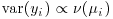, and the lack of the need to assume a specific distributional form.

If we take the original GLM density function and find the derivative of the log-likelihood with respect to the mean,

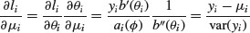
(where the primes denote differentiation), the quasi-likelihood Q is defined as

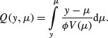
Here, the denominator is the variance of 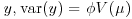, where is called the scale parameter (or the dispersion parameter) and is the variance function. We need only specify the two moments (mean μ and variance and maximize Q to find the MQL estimates of the parameters.

The scale parameter is estimated from the generalized Pearson statistic rather than from the residual deviance (as when correcting for overdispersion with Poisson or binomial errors):

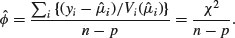
For normally distributed data, the residual sum of squares SSE is chi-squared distributed.

13.8 The quasi family of models

Instead of transforming the response variable in different ways, we can analyse the untransformed response variable but specify different link functions. This has the considerable advantage that the models are comparable by anova because they all have the same response variable. Recall that if we transform the response variable in different ways (e.g. log in one case, cube root in another case) then we cannot compare the resulting models using anova. Here are the timber data that we analysed on p. 401:

data<-read.table("c:\\temp\\timber.txt",header=T)

attach(data)

head(data)

	volume		girth	height

1	0.7458		66.23	21.0

2	0.7458		68.62	19.5

3	0.7386		70.22	18.9

4	1.1875		83.79	21.6

5	1.3613		85.38	24.3

6	1.4265		86.18	24.9

Models 1 and 2 fit the same explanatory variables,

volume∼girth+height

but use a different link function in each case: model1 uses the cube root link (this is specified as power(0.333)), model2 uses the log link. These different link functions are fitted in glm using the quasi family (this stands for ‘quasi-likelihood’):

model1 <- glm(volume∼girth+height,family=quasi(link=power(0.3333)))

model2 <- glm(volume∼girth+height,family=quasi(link=log))

The beauty of this approach is that we can now compare the models using anova because they both have the same response variable (i.e. untransformed volume):

anova(model1,model2)

Analysis of Deviance Table

Model 1: volume ∼ girth + height

Model 2: volume ∼ girth + height

 Resid. Df Resid. Dev Df Deviance

1	28 0.96554

2	28 1.42912	0 -0.46357

Both models have the same number of degrees of freedom, so there is no F test to do, but the anova function shows us the difference in deviance between the two models. The cube root link is better than the log link (residual deviance of 0.966 compared with 1.429). Note that the anova table gives us no indication of how the two models differ from one another in their link functions, so we need to be very careful in our book-keeping. We should assess the constancy-of-variance and normality-of-errors assumptions of the two models:

plot(model1)

plot(model2)

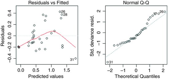
It is clear that model1 much better behaved in terms of its assumptions as well as having the lower deviance.

13.9 Generalized additive models

Generalized additive models (GAMs) are like GLMs in that they can have different error structures and different link functions to deal with count data or proportion data. What makes them different is that the shape of the relationship between y and a continuous variable x is not specified by some explicit functional form. Instead, non-parametric smoothers are used to describe the relationship. This is especially useful for relationships that exhibit complicated shapes, such as hump-shaped curves (see p. 675). The model looks just like a GLM, except that the relationships we want to be smoothed are prefixed by s: thus, if we had a three-variable multiple regression (with three continuous explanatory variables w, x and z) on count data and we wanted to smooth all three explanatory variables, we would write:

model <- gam(y∼s(w)+s(x)+s(z),poisson)

These are hierarchical models, so the inclusion of a high-order interaction (such as A:B:C) necessarily implies the inclusion of all the lower-order terms marginal to it (i.e. A:B, A:C and B:C, along with main effects for A, B and C).

Because the models are nested, the more complicated model will necessarily explain at least as much of the variation as the simpler model (and usually more). What we want to know is whether the extra parameters in the more complex model are justified in the sense that they add significantly to the models explanatory power. If they do not, then parsimony requires that we accept the simpler model.

13.10 Offsets

An offset is a component of the linear predictor that is known in advance (typically from theory, or from a mechanistic model of the process) and, because it is known, requires no parameter to be estimated from the data. For linear models with normal errors an offset is redundant, since you can simply subtract the offset from the values of the response variable, and work with the residuals instead of the y values. For GLMs, however, it is necessary to specify the offset; this is held constant while other explanatory variables are evaluated. Here is an example from the famous timber data.

The background theory is simple. We assume the logs are roughly cylindrical (i.e. that taper is negligible between the bottom and the top of the log). Then volume, v, in relation to girth, g, and height, h, is given by

Taking logarithms gives

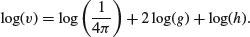
We would expect, therefore, that if we did a multiple linear regression of log(v) on log(h) and log(g) we would get estimated slopes of 1.0 for log(h) and 2.0 for log(g). Let us see what happens:

data <- read.delim("c:\\temp\\timber.txt")

attach(data)

names(data)

[1] "volume" "girth" "height"

The girths are in centimetres but all the other data are in metres, so we convert the girths to metres at the outset:

girth <- girth/100

Now fit the model:

model1 <- glm(log(volume)∼log(girth)+log(height))

summary(model1)

Coefficients:

		Estimate Std. Error t value Pr(>|t|)

(Intercept)	-2.89938	0.63767		-4.547	9.56e-05 ***

log(girth)	1.98267		0.07503		26.426	< 2e-16 ***

log(height)	1.11714		0.20448		5.463	7.83e-06 ***

The estimates are reasonably close to expectation (1.117 14 rather than 1.0 for log(h) and 1.982 67 rather than 2.0 for log(g)).

Now we shall use offset to specify the theoretical response of log(v) to log(h), i.e. a slope of 1.0 rather than the estimated 1.117 14:

model2 <- glm(log(volume)∼log(girth)+offset(log(height)))

summary(model2)

Coefficients:

		Estimate Std. Error t value Pr(>|t|)

(Intercept)	-2.53419	0.01457	-174.0	<2e-16 ***

log(girth)	2.00545		0.06287	31.9	<2e-16 ***

Naturally the residual deviance is greater, but only by a very small amount. The AIC has gone down from –62.697 to –64.336, so the model simplification was justified.

Let us try including the theoretical slope (2.0) for log(g) in the offset as well:

model3 <- glm(log(volume)∼1+offset(log(height)+2*log(girth)))

summary(model3)

Coefficients:

		Estimate Std. Error t value Pr(>|t|)

(Intercept)	-2.53403	0.01421		-178.3	<2e-16 ***

(Dispersion parameter for gaussian family taken to be 0.006259057)

 

	Null deviance: 0.18777 on 30 degrees of freedom

Residual deviance:	0.18777 on 30 degrees of freedom

AIC: -66.328

Again, the residual deviance is only marginally greater, and AIC is smaller, so the simplification is justified.

What about the intercept? If our theoretical model of cylindrical logs is correct then the intercept should be

log(1/(4*pi))

[1] -2.531024

This is almost exactly the same as the intercept estimated by GLM in model3, so we are justified in putting the entire model in the offset and informing GLM not to estimate an intercept from the data (y ∼ -1):

This is a rather curious model with no estimated parameters, but it has a residual deviance of just 0.188 05 (compared with model1, where all three parameters were estimated from the data, which had a deviance of 0.185 55). Because we were saving one degree of freedom with each step in the procedure, AIC became smaller with each step, justifying all of the model simplifications. These logs are cylindrical, not tapered as alleged in some analyses of these data.

13.11 Residuals

After fitting a model to data, we should investigate how well the model describes the data. In particular, we should look to see if there are any systematic trends in the goodness of fit. For example, does the goodness of fit increase with the observation number, or is it a function of one or more of the explanatory variables? We can work with the raw residuals:

With normal errors, the identity link, equal weights and the default scale factor, the raw and standardized residuals are identical. The standardized residuals are required to correct for the fact that with non-normal errors (like count or proportion data) we violate the fundamental assumption that the variance is constant (p. 490) because the residuals tend to change in size as the mean value the response variable changes.

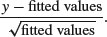
For Poisson errors, the standardized residuals are

For binomial errors they are

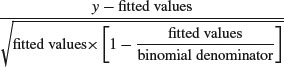
where the binomial denominator is the size of the sample from which the y successes were drawn. For gamma errors they are

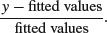
In general, we can use several kinds of standardized residuals

where the prior weights are optionally specified by you to give individual data points more or less influence (see p. 463), the scale parameter measures the degree of overdispersion (see p. 592), and the variance function describes the relationship between the variance and the mean (e.g. equality for a Poisson process; see Table 13.1).

13.11.1 Misspecified error structure

A common problem with real data is that the variance increases with the mean. The assumption in previous chapters has been of normal errors with constant variance at all values of the response variable. For continuous measurement data with non-constant errors we can specify a generalized linear model with gamma errors. These are discussed in Chapter 27 along with worked examples, and we need only note at this stage that they assume a constant coefficient of variation (see Taylor's power law, p. 262).

With count data, we often assume Poisson errors, but the data may exhibit overdispersion (see below and p. 592), so that the variance is actually greater than the mean (rather than equal to it, as assumed by the Poisson distribution). An important distribution for describing aggregated data is the negative binomial. While R has no direct facility for specifying negative binomial errors, we can use quasi-likelihood to specify the variance function in a GLM with family = quasi (see p. 564).

13.11.2 Misspecified link function

Although each error structure has a canonical link function associated with it (see p. 560), it is quite possible that a different link function would give a better fit for a particular model specification. For example, in a GLM with normal errors we might try a log link or a reciprocal link using quasi to improve the fit (for examples, see p. 563). Similarly, with binomial errors we might try a complementary log-log link instead of the default logit link function (see p. 651).

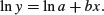
An alternative to changing the link function is to transform the values of the response variable. The important point to remember here is that changing the scale of y will alter the error structure and this will make it difficult to compare one model with another. Thus, if you take logs of y and carry out regression with normal errors, then you will be assuming that the errors in y were lognormally distributed. This may well be a sound assumption, but a bias will have been introduced if the errors really were additive on the original scale of measurement. If, for example, theory suggests that there is an exponential relationship between y and x,

then it would be reasonable to suppose that the log of y would be linearly related to x:

Now suppose that the errors ɛ in y are multiplicative with a mean of 0 and constant variance, like this:

Then they will also have a mean of 0 in the transformed model. But if the errors are additive,

then the error variance in the transformed model will depend upon the expected value of y. In a case like this, it is much better to analyse the untransformed response variable and to employ the log link function, because this retains the assumption of additive errors.

When both the error distribution and functional form of the relationship are unknown, there is no single specific rationale for choosing any given transformation in preference to another. The aim is pragmatic, namely to find a transformation that gives:

• constant error variance;
• approximately normal errors;
• additivity;
• a linear relationship between the response variables and the explanatory variables;
• straightforward scientific interpretation.

The choice is bound to be a compromise and, as such, is best resolved by quantitative comparison of the deviance produced under different model forms (see p. 270).

13.12 Overdispersion

Overdispersion is the polite statistician's version of Murphy's law: if something can go wrong, it will. Overdispersion can be a problem when working with Poisson or binomial errors, and tends to occur because you have not measured one or more of the factors that turn out to be important. It may also result from the underlying distribution being non-Poisson or non-binomial. This means that the probability you are attempting to model is not constant within each cell, but behaves like a random variable. This, in turn, means that the residual deviance is inflated. In the worst case, all the predictor variables you have measured may turn out to be unimportant so that you have no information at all on any of the genuinely important predictors. In this case, the minimal adequate model is just the overall mean, and all your ‘explanatory’ variables provide no extra information.

The techniques of dealing with overdispersion are discussed in detail when we consider Poisson errors (p. 592) and binomial errors (p. 664). Here it is sufficient to point out that there are two general techniques available to us:

• use F tests with an empirical scale parameter instead of chi-squared;
• use quasi-likelihood to specify a more appropriate variance function.

It is important, however, to stress that these techniques introduce another level of uncertainty into the analysis. Overdispersion happens for real, scientifically important reasons, and these reasons may throw doubt upon our ability to interpret the experiment in an unbiased way. It means that something we did not measure turned out to have an important impact on the results. If we did not measure this factor, then we have no confidence that our randomization process took care of it properly and we may have introduced an important bias into the results.

13.13 Bootstrapping a GLM

There are two contrasting ways of using bootstrapping with statistical models:

• Fit the model lots of times by selecting cases for inclusion at random with replacement, so that some data points are excluded and others appear more than once in any particular model fit.
• Fit the model once and calculate the residuals and the fitted values, then shuffle the residuals lots of times and add them to the fitted values in different permutations, fitting the model to the many different data sets.

In both cases, you will obtain a distribution of parameter values for the model from which you can derive confidence intervals. Here we use the timber data (a multiple regression with two continuous explanatory variables, introduced on p. 566) to illustrate the two approaches (see p. 349 for an introduction to the bootstrap).

library(boot)

The GLM model with its parameter estimates and standard errors is on p. 566. The hard part of using boot is writing the sampling function correctly. It has at least two arguments: the first must be the data on which the resampling is to be carried out (in this case, the whole dataframe called trees), and the second must be the index (the randomized subscripts showing which data values are to be used in a given realization; some cases will be repeated, others will be omitted). Inside the function we create a new dataframe based on the randomly selected indices, then fit the model to this new data set. Finally, the function should return the coefficients of the model. Here is the ‘statistic’ function in full:

model.boot <- function(data,indices){

sub.data <- data[indices,]

model <- glm(log(volume)∼log(girth)+log(height),data=sub.data)

coef(model) }

Now run the bootstrap for 2000 resamplings using the boot function:

glim.boot <- boot(trees,model.boot,R=2000)

glim.boot

ORDINARY NONPARAMETRIC BOOTSTRAP

Call:

boot(data = trees, statistic = model.boot, R = 2000)

Bootstrap Statistics:

		original	bias	std. error

t1*	-2.899379	-0.046089511	0.6452832

t2*	1.982665	-0.001071986	0.0603073

t3*	1.117138	0.014858487	0.2082793

There is very little bias in any of the three parameters, and the bootstrapped standard errors are close to their parametric estimates.

The other way of bootstrapping with a model, mentioned above, is to include all the original cases (rather than a subset of them with repeats, as we did above) but to randomize the residuals that are associated with each case. The raw residuals are y - fitted(model) and it is these values that are shuffled and allocated to cases at random. The model is then refitted and the coefficients extracted. The new y values, therefore, are

fitted(model)+ sample(y - fitted(model))

Here is a home-made version:

model <- glm(log(volume)∼log(girth)+log(height))

yhat <- fitted(model)

residuals <- log(volume) - yhat

coefs <- numeric(6000)

coefs <- matrix(coefs,nrow=2000)

We shuffle the residuals 2000 times to get different vectors of y values:

for (i in 1:2000){

y <- yhat+sample(residuals)

boot.model <- glm(y∼log(girth)+log(height))

coefs[i,] <- coef(boot.model) }

Extracting the means and standard deviations of the coefficients using apply gives:

apply(coefs,2,mean)

[1] -2.898088 1.982693 1.116724

apply(coefs,2,sd)

[1] 0.60223281 0.07231379 0.19317107

These values are close to the estimates obtained by other means earlier. Next, we use the packaged boot function to carry out the same method. The preliminaries involve fitting the GLM and extracting the fitted values (yhat), which will be the same each time, and the residuals (resids), which will be independently shuffled each time:

model <- glm(log(volume)∼log(girth)+log(height))

yhat <- fitted(model)

resids <- resid(model)

Now make a dataframe that will be fed into the bootstrap, containing the residuals to be shuffled, along with the two explanatory variables:

res.data <- data.frame(resids,girth,height)

Now for the only hard part: writing the ‘statistic’ function to do the work within boot. The first argument is always the dataframe and the second is always the index i, which controls the shuffling:

bf <- function(res.data,i) {

y <- yhat+res.data[i,1]

nd <- data.frame(y,girth,height)

model <- glm(y∼log(girth)+log(height),data=nd)

coef(model) }

Inside the function we create a particular vector of y values by adding the shuffled residuals res.data[i,1] to the fitted values, then put this vector, y, along with the explanatory variables into a new dataframe nd that will be different each time GLM the is fitted. The function returns the three coefficients from the particular fitted model, coef(model); the coefficients are the ‘statistics’ of the bootstrap, hence the name of the function.

Finally, because we want to shuffle the residuals rather than sample them with replacement, we specify sim="permutation" in the call to the boot function:

boot(res.data, bf, R=2000, sim="permutation")

DATA PERMUTATION

Call:

boot(data = res.data, statistic = bf, R = 2000, sim = "permutation")

Bootstrap Statistics :

	original	 bias		std. error

t1*	-2.899379	0.014278399	0.62166875

t2*	1.982665	0.001601178	0.07064475

t3*	1.117138	-0.004586529	0.19938992

Again, the parameter values and their standard errors are very close to those obtained by our other bootstrapping methods. Here are the confidence intervals for the three parameters, specified by index=1 for the intercept, index=2 for the slope of the regression on log(g) and index=3 for the slope of the regression on log(h):

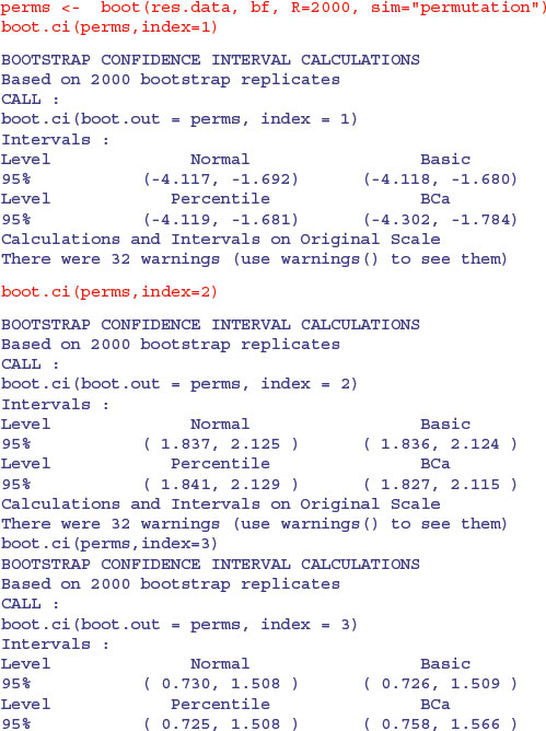
You can see that all the intervals for the slope on log(g) include the value 2.0 and all the intervals for the slope on log(h) include 1.0, consistent with the theoretical expectation that the logs are cylindrical, and that the volume of usable timber can be estimated from the length of the log and the square of its girth.

13.14 Binomial GLM with ordered categorical variables

Ordered factors are introduced on p. 443. Here is a worked example using the built-in oesophageal cancer dataframe called esoph. The response is the number of cancer cases and the matching number of non-cancer patients (controls), with three categorical explanatory variables: age group (agegp, with six ordered levels each spanning 10 years), alcohol consumption (alcgp, with four ordered levels) and tobacco consumption (tobgp, with four ordered levels). There are too few cases to fit a full factorial of agegp*tobgpacco*alcgp, so we start with a maximal model that has a main effect for age and an interaction between tobacco and alcohol:

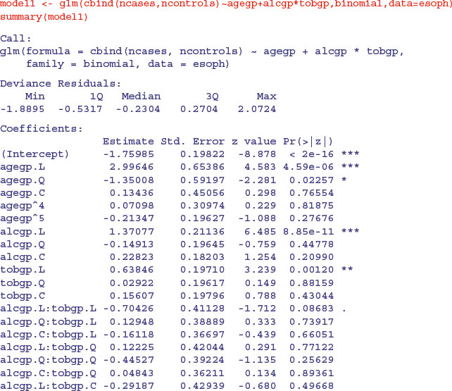
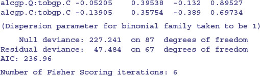
The good news is that there is no overdispersion (residual deviance 47.484 on 67 d.f.) so we can begin model simplification. You may not be familiar with the way that ordered factor levels are displayed in the summary.glm table: L means ‘linear’ testing whether there is evidence for a straight-line relationship with the response variable (look at the sign to see if it is increasing or decreasing); Q means ‘quadratic’ testing whether there is evidence for curvature in the response (look at the sign to see if the curvature is U-shaped or upside-down U-shaped); C means ‘cubic’ testing whether there is evidence for a point of inflection in the relationship; and numbers like ^4, ^5 (etc) test for higher-order polynomial effects, like local maxima and local minima in the relationship. We shall not interpret the output until we have finished with model simplification. There is no indication of an interaction between smoking and drinking, so we remove this:

model2<-glm(cbind(ncases,ncontrols)∼agegp+alcgp+tobgp,binomial,data=esoph)

anova(model1,model2)

Analysis of Deviance Table

 

Model 1: cbind(ncases, ncontrols) ∼ agegp + alcgp * tobgp

Model 2: cbind(ncases, ncontrols) ∼ agegp + alcgp + tobgp

 Resid. Df Resid. Dev Df Deviance

1	67 47.484

2	76 53.973 -9 -6.4895

The critical value of chi-squared with 9 d.f. is 16.92:

qchisq(.95,9)

[1] 16.91898

Our relatively low value of 6.4895 therefore indicates that this model simplification was justified. What next?

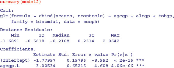
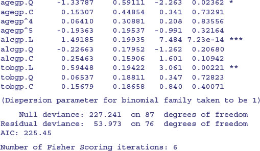
There is strong evidence for linear effects of alcohol and tobacco consumption, with a quadratic (decelerating positive) effect of age on cancer risk. The quadratic and higher-order polynomials are not significant for either tobacco or alcohol, so this is a good stage at which to consider factor-level reduction.

Let us look at the data as proportions:

p<-ncases/(ncases+ncontrols)

Now plot this against the three explanatory variables

par(mfrow=c(2,2))

plot(p∼alcgp,col="red")

plot(p∼tobgp,col="blue")

plot(p∼agegp,col="green")

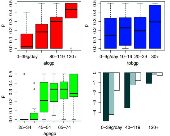
The plot suggests some sensible model simplifications (ignore the grey barplot for the moment). The alcohol response (red) looks to be linear, so we leave that as it is. The tobacco response (blue) could probably be simplified by combining the two intermediate smoking rates:

tob2<-tobgp

levels(tob2)[2:3]<-"10-30"

levels(tob2)

[1] "0-9g/day" "10-30" "30+"

The age effect is most complicated, but a three-level factor might work just as well with a young group (under age 45), an intermediate group (age between 45 and 54) and an older group (55+):

age2<-agegp

levels(age2)[4:6]<-"55+"

levels(age2)[1:2]<-"under45"

levels(age2)

[1] "under45" "45-54" "55+"

We can start the modelling again with these new ordered factors:

model3 <- glm(cbind(ncases,ncontrols)∼age2*alcgp*tob2,binomial,data=esoph)

model4<-step(model3)

model5<-update(model4,∼.-age2:alcgp)

anova(model4,model5,test="Chi")

Analysis of Deviance Table

 

Model 1: cbind(ncases, ncontrols) ∼ age2 + alcgp + tob2 + age2:alcgp

Model 2: cbind(ncases, ncontrols) ∼ age2 + alcgp + tob2

 Resid. Df Resid. Dev Df Deviance Pr(>Chi)

1	74 44.677

2	80 60.388 -6 -15.711 0.01539 *

At this stage, the ordering of the factors is more of a hindrance than a help, because it is so hard to interpret the significant age by alcohol interaction. Let us also get rid of the apparently problematical alcohol group (look at the size of its standard error in summary(model4)),

levels(alc3)[2:3]<-"40-119"

alc3<-factor(alc3,ordered=FALSE)

levels(alc3)

1] "0-39g/day" "40-119" "120+"

and unorder the other two factors for good measure:

age3<-factor(age2,ordered=FALSE)

tob3<-factor(tob2,ordered=FALSE)

We start the modelling again with a full factorial of the three unordered factors, then use step to simplify it:

model6 <- glm(cbind(ncases,ncontrols)∼age3*alc3*tob3,binomial,data=esoph)

model7<-step(model6)

summary(model7)

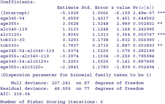
The interaction between age and alcohol is not obviously significant, so we test it by deletion:

model8<-update(model7,∼.-age3:alc3)

anova(model7,model8,test="Chi")

Analysis of Deviance Table

 

Model 1: cbind(ncases, ncontrols) ∼ age3 + alc3 + tob3 + age3:alc3

Model 2: cbind(ncases, ncontrols) ∼ age3 + alc3 + tob3

 Resid. Df Resid. Dev Df Deviance Pr(>Chi)

1	77 48.559

2	81 62.468 -4 -13.909 0.00759 **

It turns out that the interaction is highly significant (p < 0.008). To visualize the interaction, we plot the predicted means of the logits by age and alcohol consumption:

barplot(tapply(predict(model7),list(age3,alc3),mean),beside=T)

This is the grey-scale barplot in the lower right-hand panel, above. The young and middle-aged subjects both have low rates of cancer at low alcohol consumption rates, but the middle-aged subjects have proportionally higher rates at intermediate alcohol consumption and, by the highest rates of alcohol consumption, the two older age classes have equally high rates of cancer. Again, the interaction has become clear only after model simplification.