Chapter 17
Binary Response Variables
Many statistical problems involve binary response variables. For example, we often classify individuals as
- dead or alive,
- occupied or empty,
- healthy or diseased,
- wilted or turgid,
- male or female,
- literate or illiterate,
- mature or immature,
- solvent or insolvent, or
- employed or unemployed.
It is interesting to understand the factors that are associated with an individual being in one class or the other. Binary analysis will be a useful option when at least one of your explanatory variables is continuous (rather than categorical). In a study of company insolvency, for instance, the data would consist of a list of measurements made on the insolvent companies (their age, size, turnover, location, management experience, workforce training, and so on) and a similar list for the solvent companies. The question then becomes which, if any, of the explanatory variables increase the probability of an individual company being insolvent.
The response variable contains only 0s and 1s; for example, 0 to represent dead individuals and 1 to represent live ones. Thus, there is only a single column of numbers for the response, in contrast to proportion data where two vectors (successes and failures) were bound together to form the response (see Chapter 16). The way that R treats binary data is to assume that the 0s and 1s come from a binomial trial with sample size 1. If the probability that an individual is dead is p, then the probability of obtaining y (where y is either dead or alive, 0 or 1) is given by an abbreviated form of the binomial distribution with n = 1, known as the Bernoulli distribution:
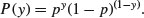
The random variable y has a mean of p and a variance of p(1 – p), and the objective is to determine how the explanatory variables influence the value of p. The trick to using binary response variables effectively is to know when it is worth using them, and when it is better to lump the successes and failures together and analyse the total counts of dead individuals, occupied patches, insolvent firms or whatever. The question you need to ask yourself is: do I have unique values of one or more explanatory variables for each and every individual case?
If the answer is ‘yes’, then analysis with a binary response variable is likely to be fruitful. If the answer is ‘no’, then there is nothing to be gained, and you should reduce your data by aggregating the counts to the resolution at which each count does have a unique set of explanatory variables. For example, suppose that all your explanatory variables were categorical – sex (male or female), employment (employed or unemployed) and region (urban or rural). In this case there is nothing to be gained from analysis using a binary response variable because none of the individuals in the study have unique values of any of the explanatory variables. It might be worthwhile if you had each individual's body weight, for example; then you could ask whether, when you control for sex and region, heavy people are more likely to be unemployed than light people. In the absence of unique values for any explanatory variables, there are two useful options:
- Analyse the data as a contingency table using Poisson errors, with the count of the total number of individuals in each of the eight contingencies (2×2×2) as the response variable (see Chapter 15) in a dataframe with just eight rows.
- Decide which of your explanatory variables is the key (perhaps you are interested in gender differences), then express the data as proportions (the number of males and the number of females) and recode the binary response as a count of a two-level factor. The analysis is now of proportion data (the proportion of all individuals that are female, for instance) using binomial errors (see Chapter 16).
If you do have unique measurements of one or more explanatory variables for each individual, these are likely to be continuous variables such as body weight, income, medical history, distance to the nuclear reprocessing plant, geographic isolation, and so on. This being the case, successful analyses of binary response data tend to be multiple regression analyses or complex analyses of covariance, and you should consult Chapters 10 and 12 for details on model simplification and model criticism.
In order to carry out modelling on a binary response variable we take the following steps:
- Create a single vector containing 0s and 1s as the response variable.
- Use glm with family=binomial.
- Consider changing the link function from the default logit to complementary log-log.
- Fit the model in the usual way.
- Test significance by deletion of terms from the maximal model, and compare the change in deviance with chi-squared.
Note that there is no such thing as overdispersion with a binary response variable, and hence no need to change to using quasibinomial when the residual deviance is large. The choice of link function is generally made by trying both links and selecting the link that gives the lowest deviance. The logit link that we used earlier is symmetric in p and q, but the complementary log-log link is asymmetric. You may also improve the fit by transforming one or more of the explanatory variables. Bear in mind that you can fit non-parametric smoothers to binary response variables using generalized additive models (as described in Chapter 18) instead of carrying out parametric logistic regression.
17.1 Incidence functions
In this example, the response variable is called incidence; a value of 1 means that an island was occupied by a particular species of bird, and 0 means that the bird did not breed there. The explanatory variables are the area of the island (km2) and the isolation of the island (distance from the mainland, km).
island <- read.table("c:\\temp\\isolation.txt",header=T)

attach(island)

names(island)
[1] "incidence" "area" "isolation"
There are two continuous explanatory variables, so the appropriate analysis is multiple regression. The response is binary, so we shall do logistic regression with binomial errors.
We begin by fitting a complex model involving an interaction between isolation and area:
model1 <- glm(incidence∼area*isolation,binomial)
Then we fit a simpler model with only main effects for isolation and area:
model2 <- glm(incidence∼area+isolation,binomial)
We now compare the two models using ANOVA:
anova(model1,model2,test="Chi")
Analysis of Deviance Table


Model 1: incidence ∼ area * isolation

Model 2: incidence ∼ area + isolation

 Resid. Df Resid.	Dev Df Deviance Pr(>Chi)

1		46		28.252

2		47		28.402 -1 -0.15043	0.6981
The simpler model is not significantly worse, so we accept this for the time being, and inspect the parameter estimates and standard errors:
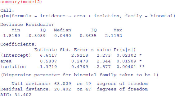
The estimates and their standard errors are in logits. We see that area has a significant positive effect (larger islands are more likely to be occupied), but isolation has a very strong negative effect (isolated islands are much less likely to be occupied). This is the minimal adequate model. We should plot the fitted model through the scatterplot of the data. It is much easier to do this for each variable separately, like this:
modela <- glm(incidence∼area,binomial)

modeli <- glm(incidence∼isolation,binomial)


windows(7,4)

par(mfrow=c(1,2))


xv <- seq(0,9,0.01)

yv <- predict(modela,list(area=xv),type="response")

plot(area,incidence)

lines(xv,yv, col="red")


xv2 <- seq(0,10,0.01)

yv2 <- predict(modeli,list(isolation=xv2),type="response")

plot(isolation,incidence)

lines(xv2,yv2, col="red")

17.2 Graphical tests of the fit of the logistic to data
The logistic plots above are all well and good, but it is very difficult to know how good the fit of the model is when the data are shown only as 0s or 1s. Some people have argued for putting histograms instead of rugs on the top and bottom axes, but there are issues here about the arbitrary location of the bins (see p. 279). Rugs are a one-dimensional addition to the bottom (or top) of the plot showing the locations of the data points along the x axis. The idea is to indicate the extent to which the values are clustered at certain values of the explanatory variable, rather than evenly spaced out along it. If there are many values at the same value of x, it will be useful to use the jitter function to spread them out (by randomly selected small distances from x).
A different tack is to cut the data into a number of sectors and plot empirical probabilities (ideally with their standard errors) as a guide to the fit of the logistic curve, but this, too, can be criticized on the arbitrariness of the boundaries to do the cutting, coupled with the fact that there are often too few data points to give acceptable precision to the empirical probabilities and standard errors in any given group.
For what it is worth, here is an example of this approach. The response is occupation of territories and the explanatory variable is resource availability in each territory:
occupy <- read.table("c:\\temp\\occupation.txt",header=T)

attach(occupy)

names(occupy)
[1] "resources" "occupied"
plot(resources,occupied,type="n")

rug(jitter(resources[occupied==0]))

rug(jitter(resources[occupied==1]),side=3)
Now fit the logistic regression and draw the line:
model <- glm(occupied∼resources,binomial)

xv <- 0:1000

yv <- predict(model,list(resources=xv),type="response")

lines(xv,yv,col="red")
The idea is to cut up the ranked values on the x axis (resources) into five categories and then work out the mean and the standard error of the proportions in each group:

If you have not met the cut function before, you will be impressed. It has taken the continuous variable called resources, and cut it up into five bins in creating a factor called cutr. The margins of the bins are defined within curved and square brackets which are read as follows: (13.2, 209] means ‘from, but not including, 13.2 to, and including, 209’. So the figure next to the round bracket is excluded from this bin and is included in the adjacent bin (to the left in this case). This option is called right=TRUE and is the default for cut. We use the table function to count the number of cases in each bin:
table(cutr)
cutr

	(13.2,209] (209,405] (405,600] (600,796] (796,992]

	 31	 29	 30	 29	 31
So the empirical probabilities are given by:
probs <- tapply(occupied,cutr,sum)/table(cutr)

probs
(13.2,209]	(209,405]	(405,600]	(600,796]	(796,992]

 0.0000000 0.3448276	0.8333333	0.8965517	1.0000000
probs <- as.vector(probs)

resmeans <- tapply(resources,cutr,mean)

resmeans <- as.vector(resmeans)
We can plot these as big points on the graph – the closer they fall to the line, the better the fit of the logistic model to the data:
points(resmeans,probs,pch=16,cex=2,col="blue")
We need to add a measure of unreliability to the points. The standard error of a binomial proportion will do:  .
.
se <- sqrt(probs*(1-probs)/table(cutr))
Finally, draw lines up and down from each point indicating one standard error:
up <- probs+as.vector(se)

down <- probs-as.vector(se)


for (i in 1:5) {

 	lines(c(resmeans[i],resmeans[i]),c(up[i],down[i]), col="blue") }
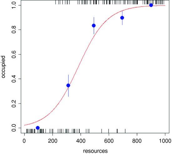
Evidently, the logistic is a good fit to the data above resources of 800 (not surprising, though, given that there were no unoccupied patches in this region), but it is rather a poor fit for resources between 400 and 800, as well as below 200, despite the fact that there were no occupied patches in the latter region (empirical p = 0).
17.3 ANCOVA with a binary response variable
In our next example the binary response variable is parasite infection (infected or not) and the explanatory variables are weight and age (continuous) and sex (categorical). We begin with data inspection:
infection <- read.table("c:\\temp\\infection.txt",header=T)

attach(infection)

names(infection)
[1] "infected" "age" "weight" "sex"
windows(7,4)

par(mfrow=c(1,2))

plot(infected,weight,xlab="Infection",ylab="Weight",col="green")

plot(infected,age,xlab="Infection",ylab="Age",col="green4")

Infected individuals are substantially lighter than uninfected individuals, and occur in a much narrower range of ages. To see the relationship between infection and gender (both categorical variables) we can use table:
table(infected,sex)
	sex

infected	female	male

 absent	17	47

 present	11	6
This indicates that the infection is much more prevalent in females (11/28) than in males (6/53).
We now proceed, as usual, to fit a maximal model with different slopes for each level of the categorical variable:
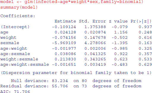
It certainly does not look as if any of the high-order interactions are significant. Instead of using update and anova for model simplification, we can use step to compute the AIC for each term in turn:
model2 <- step(model)
Start: AIC=71.71
First, it tests whether the three-way interaction is required:
infected ∼ age * weight * sex


		Df Deviance	AIC

- age:weight:sex	1	55.943 69.943

<none>			55.706 71.706
This causes a reduction in AIC of just 71.7 – 69.9 = 1.8 and hence is not significant. Next, it looks at the three two-way interactions and decides which to delete first:
Step: AIC=69.94
		Df Deviance	AIC

- weight:sex	1	56.122 68.122

- age:sex	1		 57.828 69.828

<none>			55.943 69.943

- age:weight	1	58.674 70.674
Only the removal of the weight–sex interaction causes a reduction in AIC, so this interaction is deleted and the other two interactions are retained. Let us see if we would have been this lenient:

Neither of the two interactions retained by step would figure in our model (p > 0.10). We shall use update to simplify model2:
model3 <- update(model2,∼.-age:weight)

anova(model2,model3,test="Chi")
Analysis of Deviance Table


Model 1: infected ∼ age + weight + sex + age:weight + age:sex

Model 2: infected ∼ age + weight + sex + age:sex

 Resid. Df Resid.	Dev Df Deviance Pr(>Chi)

1	75	56.122

2	76	58.899 -1	-2.777	0.09562 .
So there is no really persuasive evidence of an age–weight term (p = 0.096).
model4 <- update(model2,∼.-age:sex)

anova(model2,model4,test="Chi")
Analysis of Deviance Table


Model 1: infected ∼ age + weight + sex + age:weight + age:sex
Model 2: infected ∼ age + weight + sex + age:weight

 Resid. Df Resid. Dev Df Deviance Pr(>Chi)

1	75	56.122

2	76	58.142 -1	-2.0203		0.1552
Note that we are testing all the two-way interactions by deletion from the model that contains all two-way interactions (model2): p = 0.1552, so nothing there, then.
What about the three main effects?
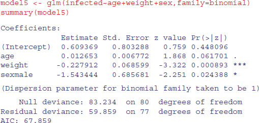
Weight is highly significant, as we expected from the initial boxplot, sex is quite significant, and age is marginally significant. It is worth establishing whether there is any evidence of non-linearity in the response of infection to weight or age. We might begin by fitting quadratic terms for the two continuous explanatory variables:
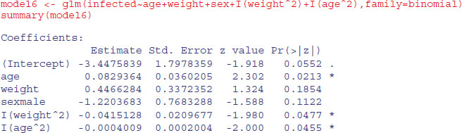

Evidently, both relationships are significantly curvilinear. It is worth looking at these non-linearities in more detail, to see if we can do better with other kinds of models (e.g. non-parametric smoothers, piecewise linear models or step functions). A generalized additive model is often a good way to start when we have continuous covariates:
library(mgcv)

model7 <- gam(infected∼sex+s(age)+s(weight),family=binomial)

windows(7,4)

par(mfrow=c(1,2))

plot.gam(model7)
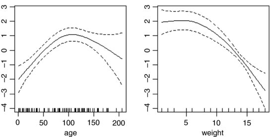
These non-parametric smoothers are excellent at showing the humped relationship between infection and age, and at highlighting the possibility of a threshold at weight ≈ 8 in the relationship between weight and infection. We can now return to a GLM to incorporate these ideas. We shall fit age and age2 as before, but try a piecewise linear fit for weight, estimating the threshold weight at a range of values (say 8–14) and selecting the threshold that gives the lowest residual deviance; this turns out to be a threshold of 12 (rather higher than suggested by the gam plot above). The piecewise regression is specified by the term:
I((weight - 12) * (weight > 12))
The I (‘as is’) is necessary to stop the * being evaluated as an interaction term in the model formula. What this expression says is ‘regress infection on the value of weight - 12, but only do this when weight > 12 is true’ (see p. 25). Otherwise, assume that infection is independent of weight.
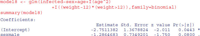
The effect of sex on infection is not quite significant (p = 0.071 for a chi-squared test on deletion), so we leave it out. The quadratic term for age does not look highly significant here, but a deletion test gives p = 0.011, so we retain it. The minimal adequate model is therefore

We conclude that there is a humped relationship between infection and age, and a threshold effect of weight on infection. The effect of sex is marginal, but might repay further investigation (p = 0.071).
17.4 Binary response with pseudoreplication
In the bacteria dataframe, which is part of the MASS library, we have repeated assessment of bacterial infection (yes or no, coded as y or n) in a series of patients allocated at random to one of three treatments: placebo, drug and drug plus supplement (drug+). The trial lasted for 11 weeks and different patients were assessed on different numbers of occasions. The question is whether the two treatments significantly reduced bacterial infection.
library(MASS)

attach(bacteria)

names(bacteria)
[1] "y" "ap" "hilo" "week" "ID" "trt"
table(y)
y

 n	y

 43	177
The data are binary, so we need to use family=binomial. There is temporal pseudoreplication (repeated measures on the same patients) so we cannot use glm. The ideal solution is the generalized mixed models function lmer. Like glm, the lmer function can take text (e.g. a two-level factor like y) as the response variable. We start by looking at the data:
table(y,trt)
 trt

y	placebo		drug	drug+

 n	12		18	13

 y	84		44	49
Preliminary data inspection suggests that the drug might be effective because only 12 out of 96 patient visits were bacteria-free in the placebos, compared with 31 out of 124 for the treated individuals. We shall see. The modelling goes like this: the lmer function is in the lme4 package. The random effects appear in the same formula as the fixed effects, but defined by the round brackets and the ‘given’ operator | to separate the continuous random effect (week) from the categorical random effect (patient ID):

Variation in intercepts across the patients (0.148) explained roughly twice as much variation in infection as did random variation in slopes (0.062). The fixed effects are not significant.
We can simplify the model by removing the dependence of infection on week, retaining only the intercept as a random effect +(1|ID):
model2 <- lmer(y∼trt+(1|ID),family=binomial)

anova(model1,model2)
Data:

Models:

model2: y ∼ trt + (1|ID)

model1: y ∼ trt + (week|ID)

	Df AIC BIC		logLik	Chisq Chi Df Pr(>Chisq)

model2	4 214.32 227.90	-103.162

model1	6 209.21 229.57	-98.603 9.1184	2	0.01047 *
The simpler model2 is significantly worse (p = 0.010 47) so we accept model1 (it has a lower AIC than model2), retaining the random effect for week.
There is a question about the factor levels: perhaps the drug effect would be more significant if we combine the drug and drug+ treatments?

The interpretation is straightforward: there is no evidence in this experiment that either treatment significantly reduces bacterial infection. Note that this is not the same as saying that the drug does not work. It is simply that this trial is too small to demonstrate the significance of its efficacy.
It is also important to appreciate the importance of the pseudoreplication. If we had ignored the fact that there were multiple measures per patient we should have concluded wrongly that the drug effect was significant. Here are the raw data on the counts:
table(y,trt)
 trt

y	placebo	drug	drug+

 n	12	18	13

 y	84	44	49
Here is the wrong way of testing for the significance of the treatment effect:
prop.test(c(12,18,13),c(96,62,62))
	3-sample test for equality of proportions without continuity correction


data: c(12, 18, 13) out of c(96, 62, 62)

X-squared = 6.6585, df = 2, p-value = 0.03582

alternative hypothesis: two.sided

sample estimates:

 prop 1	prop 2	prop 3

0.1250000 0.2903226 0.2096774
It appears that the drug has increased the rate of non-infection from 0.125 in the placebos to 0.29 in the treated patients, and that this effect is significant (p = 0.035 82). As we have seen, however, when we remove the pseudoreplication by using the appropriate mixed model with lmer the response is non-significant.
Another way to get rid of the pseudoreplication is to restrict the analysis to the patients that were there at the end of the experiment. We just use subset=(week==11) and this removes all the pseudoreplication because no subjects were measured twice within any week – we can check this with the any function:
any(table(ID,week) >1)
[1] FALSE
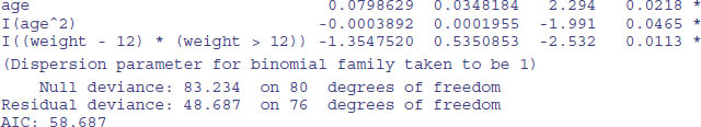
The model is a straightforward GLM with a binary response variable and a single explanatory variable (the three-level factor called trt):
Neither drug treatment has anything approaching a significant effect in lowering bacterial infection rates compared with the placebos (p = 0.4032). The supplement was expected to increase bacterial control over the drug treatment, so perhaps the interpretation will be modified lumping together the two drug treatments:
drugs <- factor(1+(trt=="placebo"))
Here are placebos plus patients getting one drug treatment or the other:
table(drugs[week==11])
 1 2

24 20
Thus there were 24 patients receiving one drug or the other, and 20 placebos (at 11 weeks).


Clearly, there is no convincing effect for the drug treatments on bacterial infection when we use this subset of the data (p = 0.327).
An alternative way of analysing all the data (including the pseudoreplication) is to ask what proportion of tests on each patient scored positive for the bacteria. The response variable now becomes a proportion, and the pseudoreplication disappears because we only have one number for each patient (i.e. a count of the number of occasions on which each patient scored positive for the bacteria, with the binomial denominator as the total number of tests on that patient).
There are some preliminary data-shortening tasks. We need to create a vector of length 50 containing the drug treatments of each patient (tss) and a table (ys, with elements of length 50) scoring how many times each patient was infected and uninfected by bacteria. Finally, we use cbind to create a two-column response variable, yv:
dss <- data.frame(table(trt,ID))

head(dss)
	trt		ID Freq

1	placebo X01	4

2	drug X01		0

3	drug+ X01		 0

4	placebo X02	0

5	drug X02		0

6	drug+ X02		 4
We need to find out the treatments of the patients that scored Freq > 0:
tss <- dss[dss[,3]>0,]$trt


ys <- table(y,ID)


yv <- cbind(ys[2,],ys[1,])
Now we can fit a very simple model for the binomial response (glm with binomial errors):

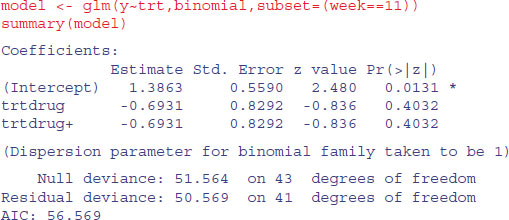
Drug looks to be significant here, but note that the residual deviance is much bigger than the residual degrees of freedom, so we should correct for overdispersion by using quasi-binomial instead of binomial errors (recall that the response is now binomial rather than binary; see p. 651):

There is a marginally significant effect of drug, but no significant difference between the two drug treatments, so we aggregate them into a single drug treatment:
Again, the treatment effect is not significant, in agreement with the generalized mixed-effects model (p. 662). This example re-emphasizes the importance of correcting for pseudoreplication and overdispersion. Had we not made allowance for these we would have concluded (wrongly) that the drug brought about significant a reduction in infection.