Chapter 18

Generalized Additive Models

Up to this point, continuous explanatory variables have been added to models as linear functions, linearized parametric transformations, or through various link functions. In all cases, an explicit or implicit assumption was made about the parametric form of the function to be fitted to the data (whether quadratic, logarithmic, exponential, logistic, reciprocal or whatever). In many cases, however, you have one or more continuous explanatory variables, but you have no a priori reason to choose one particular parametric form over another for describing the shape of the relationship between the response variable and the explanatory variable(s). Generalized additive models (GAMs) are useful in such cases because they allow you to capture the shape of a relationship between y and x without prejudging the issue by choosing a particular parametric form.

Generalized additive models (implemented in R by the gam function) extend the range of application of generalized linear models (glm) by allowing non-parametric smoothers in addition to parametric forms, and these can be associated with a range of link functions. All of the error families allowed with glm are available with gam (binomial, poisson, Gamma, etc.). Indeed, gam has many of the attributes of both glm and lm, and the output can be modified using update. You can use all of the familiar methods such as print, plot, summary, anova, predict and fitted after a GAM has been fitted to data. The gam function used in this book is in the mgcv package contributed by Simon Wood:

library(mgcv)

There are many ways of specifying the model in a GAM: all of the continuous explanatory variables x, w and z can enter the model as non-parametrically smoothed functions like this:

y∼s(x) + s(w) + s(z)

Alternatively, the model can contain a mix of parametrically estimated parameters (x and z) and smoothed variables s(w):

y∼x + s(w) + z

Formulae can involve nested (two-dimensional) terms in which the smoothing s() terms have more than one argument, implying an isotropic smooth:

y∼s(x) + s(z) + s(x,z)

Alternatively the smoothers can have overlapping terms such as

y∼s(x,z) + s(z,w)

The user has a high degree of control over the way that interactions terms can be fitted, and te() smooths are provided as an effective means for modelling smooth interactions of any number of variables via scale-invariant tensor product smooths. Here is an example of a model formula with a fully nested tensor product te(x,z,k=6):

y ∼ s(x,bs="cr",k=6) + s(z,bs="cr",k=6) + te(x,z,k=6)

The optional arguments to the smoothers are bs="cr",k=6, where bs indicates the basis to use for the smooth ("cr" is a cubic regression spline; the default is thin plate bs="tp"), and k is the dimension of the basis used to represent the smooth term (it defaults to k = 10*3(d-1) where d is the number of covariates for this term).

18.1 Non-parametric smoothers

You can see non-parametric smoothers in action for fitting a curve through a scatterplot in Chapter 10 (p. 491). Here we are concerned with using non-parametric smoothers in statistical modelling where the object is to assess the relative merits of a range of different models in explaining variation in the response variable. One of the simplest model-fitting functions is loess (which replaces its predecessor called lowess).

The following example shows population change, Delta = log(N(t+1)/N(t)), as a function of population density (N(t)) in an investigation of density dependence in a sheep population. This is what the data look like:

soay <- read.table("c:\\temp\\soaysheep.txt",header=T)

attach(soay)

names(soay)

[1] "Year" "Population" "Delta"

plot(Population,Delta,pch=21,col="green",bg="red")

Broadly speaking, population change is positive at low densities (Delta > 0) and negative at high densities (Delta < 0) but there is a great deal of scatter, and it is not at all obvious what shape of smooth function would best describe the data. Here is the default loess:

model <- loess(Delta∼Population)

summary(model)

Call:

loess(formula = Delta∼Population)

Number of Observations: 44

Equivalent Number of Parameters: 4.66

Residual Standard Error: 0.2616

Trace of smoother matrix: 5.11

Control settings:

 	normalize: TRUE

 	span :	 0.75

 	degree : 2

 	family : gaussian

 	surface :interpolate cell = 0.2

Now draw the smoothed line using predict to extract the predicted values from model:

xv <- seq(600,2000,1)

yv <- predict(model,data.frame(Population=xv))

lines(xv,yv col="red")

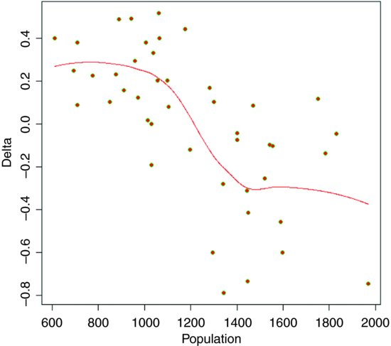
The smooth curve looks rather like a step function. We can compare this smooth function with a step function, using a tree model (p. 768) as an objective way of determining the threshold for splitting the data into low- and high-density parts:

library(tree)

thresh <- tree(Delta∼Population)

print(thresh)

The threshold for the first split of the tree model is at Population = 1289.5, so we define this as the threshold density:

th <- 1289.5

Then we can use this threshold to create a two-level factor for fitting two constant rates of population change using aov:

model2 <- aov(Delta∼(Population>th))

summary(model2)

			Df Sum Sq Mean Sq F value Pr(>F)

Population >	th 1 2.810 2.810 47.63 2.01e-08 ***

Residuals		42 2.477	 0.059 

showing a residual error variance of 0.059. This compares with the residual of 0.26162 = 0.068 from the loess (above). To draw the step function we need the average low-density population increase and the average high-density population decline:

tapply(Delta[-45],(Population[-45]>th),mean)

 FALSE		TRUE

0.2265084 -0.2836616 

Note the use of negative subscripts to drop the NA from the last value of Delta. Then use these figures to draw the step function:

lines(c(600,th),c(0.2265,0.2265),lty=2, col="blue")

lines(c(th,2000),c(-0.2837,-0.2837),lty=2, col="blue")

lines(c(th,th),c(-0.2837,0.2265),lty=2, col="blue")

It is a moot point which of these two models is the most realistic scientifically, but the step function involved three estimated parameters (two averages and a threshold), while the loess is based on 4.66 degrees of freedom, so parsimony favours the step function (it also has a slightly lower residual sum of squares).

18.2 Generalized additive models

This dataframe contains measurements of radiation, temperature, wind speed and ozone concentration. We want to model ozone concentration as a function of the three continuous explanatory variables using non-parametric smoothers rather than specified nonlinear functions (the parametric multiple regression analysis of these data is on p. 490):

ozone.data <- read.table("c:\\temp\\ozone.data.txt",header=T)

attach(ozone.data)

names(ozone.data)

[1] "rad" "temp" "wind" "ozone"

For data inspection we use pairs with a non-parametric smoother, lowess:

pairs(ozone.data, panel=function(x,y) { points(x,y); lines(lowess(x,y))} )

Now fit all three explanatory variables using the non-parametric smoother s():

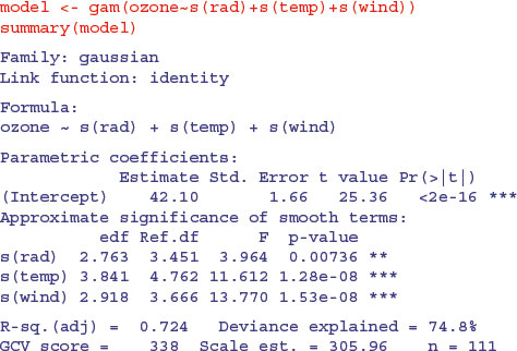
Note that the intercept is estimated as a parametric coefficient (42.10; upper table) and the three explanatory variables are fitted as smooth terms. All three are significant, but radiation is the least significant at p = 0.007 36. We can compare a GAM with and without a term for radiation using ANOVA in the normal way:

model2 <- gam(ozone∼s(temp)+s(wind))

anova(model,model2,test="F")

Analysis of Deviance Table

 	

Model 1: ozone ∼ s(rad) + s(temp) + s(wind)

Model 2: ozone ∼ s(temp) + s(wind)

 	Resid. Df Resid. Dev	Df Deviance		F Pr(>F)

1	100.48		30742

2	102.85		34885 -2.3672 -4142.2 5.7192 0.002696 **

Clearly, radiation should remain in the model, since deletion of radiation caused a highly significant increase in deviance (p = 0.0027), emphasizing the fact that deletion is a better test than inspection of parameters (the p values in the full model table were not deletion p values).

We should investigate the possibility that there is an interaction between wind and temperature:

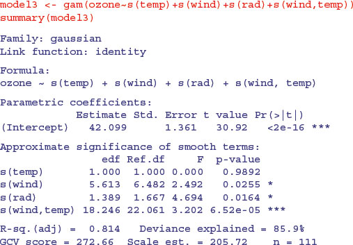
The interaction appears to be highly significant, but the main effect of temperature is cancelled out. We can inspect the fit of model3 like this:

par(mfrow=c(2,2))

plot(model3,residuals=T,pch=16)

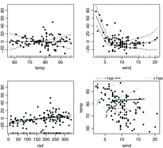
The etchings on the x axis are called rugs (see Section 17.2) and indicate the locations of measurements of x values on each axis. The default option is rug=T. The bottom right-hand plot shows the complexity of the interaction between temperature and wind speed.

18.2.1 Technical aspects

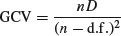
The degree of smoothness of model terms is estimated as part of fitting; isotropic or scale-invariant smooths of any number of variables are available as model terms. Confidence or credible intervals are readily available for any quantity predicted using a fitted model. In mgcv, gam solves the smoothing parameter estimation problem by using the generalized cross validation (GCV) criterion

or an unbiased risk estimator (UBRE) criterion

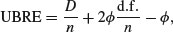
where D is the deviance, n the number of data, the scale parameter and d.f. the effective degrees of freedom of the model. Notice that UBRE is effectively just AIC rescaled, but is only used when is known. It is also possible to replace D by the Pearson statistic (see ?gam.method), but this can lead to oversmoothing. Smoothing parameters are chosen to minimize the GCV or UBRE score for the model, and the main computational challenge solved by the mgcv package is to do this efficiently and reliably. Various alternative numerical methods are provided: see ?gam.method. Smooth terms are represented using penalized regression splines (or similar smoothers) with smoothing parameters selected by GCV or UBRE or by regression splines with fixed degrees of freedom (mixtures of the two are permitted). Multi-dimensional smooths are available using penalized thin plate regression splines (isotropic) or tensor product splines (when an isotropic smooth is inappropriate).

This gam function is not a clone of what S-PLUS provides – there are three major differences. First, by default, estimation of the degree of smoothness of model terms is part of model fitting. Second, a Bayesian approach to variance estimation is employed that makes for easier confidence interval calculation (with good coverage probabilities). Third, the facilities for incorporating smooths of more than one variable are different.

If absolutely any smooth functions were allowed in model fitting then maximum likelihood estimation of such models would invariably result in complex overfitting estimates of the smoothed functions s(x) and s(z). For this reason the models are usually fitted by penalized likelihood maximization, in which the model deviance (negative log-likelihood) is modified by the addition of a penalty for each smooth function, penalizing what the author of gam, Simon Wood, calls its ‘wiggliness’. To control the trade-off between penalizing wiggliness and penalizing badness of fit, each penalty is multiplied by an associated smoothing parameter: how to estimate these parameters and how to practically represent the smooth functions are the main statistical questions introduced by moving from GLMs to GAMs.

The built-in alternatives for univariate smooths terms are: a conventional penalized cubic regression spline basis, parameterized in terms of the function values at the knots; a cyclic cubic spline with a similar parameterization; and thin plate regression splines. The cubic spline bases are computationally very efficient, but require knot locations to be chosen (automatically by default). The thin plate regression splines are optimal low-rank smooths which do not have knots, but are computationally more costly to set up. Smooths of several variables can be represented using thin plate regression splines, or tensor products of any available basis, including user-defined bases (tensor product penalties are obtained automatically form the marginal basis penalties).

Thin plate regression splines are constructed by starting with the basis for a full thin plate spline and then truncating this basis in an optimal manner, to obtain a low-rank smoother. Details are given in Wood (2003). One key advantage of the approach is that it avoids the knot placement problems of conventional regression spline modelling, but it also has the advantage that smooths of lower rank are nested within smooths of higher rank, so that it is legitimate to use conventional hypothesis testing methods to compare models based on pure regression splines. The thin plate regression spline basis can become expensive to calculate for large data sets. In this case the user can supply a reduced set of knots to use in basis construction (see knots in the argument list), or use tensor products of cheaper bases. In the case of the cubic regression spline basis, knots of the spline are placed evenly throughout the covariate values to which the term refers. For example, if fitting 101 data points with an 11-knot spline of x then there would be a knot at every 10th (ordered) x value. The parameterization used represents the spline in terms of its values at the knots. The values at neighbouring knots are connected by sections of cubic polynomial constrained to be continuous up to and including second derivatives at the knots. The resulting curve is a natural cubic spline through the values at the knots (given two extra conditions specifying that the second derivative of the curve should be zero at the two end knots). This parameterization gives the parameters a nice interpretability. Details of the underlying fitting methods are given in Wood (2000, 2004).

You must have more unique combinations of covariates than the model has total parameters (total parameters being the sum of basis dimensions plus the sum of non-spline terms less the number of spline terms.). Automatic smoothing parameter selection is not likely to work well when fitting models to very few response data. With large data sets (more than a few thousand data) the tp basis gets very slow to use: use the knots argument as discussed above and shown in the examples. Alternatively, for low-density smooths you can use the cr basis and for multi-dimensional smooths use te smooths.

For data with many zeros clustered together in the covariate space it is quite easy to set up GAMs which suffer from identifiability problems, particularly when using Poisson or binomial families. The problem is that with log or logit links, for example, mean value zero corresponds to an infinite range on the linear predictor scale.

Another situation that occurs quite often is the one in which we would like to find out if the model

is really necessary, or whether

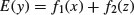
would not do just as well. One way to do this is to look at the results of fitting

y∼s(x)+s(z)+s(x,z)

gam automatically generates side conditions to make this model identifiable. You can also estimate overlapping models such as

y∼s(x,z)+s(z,v)

Sometimes models of the form

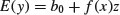
need to be estimated (where f is a smooth function, as usual). The appropriate formula is

y∼z+s(x,by=z)

where the by argument ensures that the smooth function gets multiplied by covariate z, but GAM smooths are centred (average value zero), so the parametric term for z is needed as well (f is being represented by a constant plus a centred smooth). If we wanted

then the appropriate formula would be

y∼z+s(x,by=z)-1

The by mechanism also allows models to be estimated in which the form of a smooth depends on the level of a factor, but to do this the user must generate the dummy variables for each level of the factor. Suppose, for example, that fac is a factor with three levels 1, 2, 3, and at each level of this factor the response depends smoothly on a variable x in a manner that is level-dependent. Three dummy variables, fac.1, fac.2, fac.3, can be generated for the factor (e.g. fac.1 <- as.numeric(fac==1)). Then the model formula would be:

y∼fac+s(x,by=fac.1)+s(x,by=fac.2)+s(x,by=fac.3)

In the above examples the smooths of more than one covariate have all employed single-penalty thin plate regression splines. These isotropic smooths are not always appropriate: if variables are not naturally well scaled relative to each other then it is often preferable to use tensor product smooths, with a wiggliness penalty for each covariate of the term. See ?te for examples.

The most logically consistent method to use for deciding which terms to include in the model is to compare GCV/UBRE scores for models with and without the term. More generally, the score for the model with a smooth term can be compared to the score for the model with the smooth term replaced by appropriate parametric terms. Candidates for removal can be identified by reference to the approximate p values provided by summary.gam. Candidates for replacement by parametric terms are smooth terms with estimated degrees of freedom close to their minimum possible.

18.3 An example with strongly humped data

The ethanol dataframe contains 88 sets of measurements for variables from an experiment in which ethanol was burned in a single cylinder automobile test engine. The response variable, NOx, is the concentration of nitric oxide (NO) and nitrogen dioxide (NO2) in engine exhaust, normalized by the work done by the engine, and the two continuous explanatory variables are C (the compression ratio of the engine), and E (the equivalence ratio at which the engine was run, which is a measure of the richness of the air–ethanol mix).

install.packages("SemiPar")

library(SemiPar)

data(ethanol)

attach(ethanol)

head(ethanol)

	NOx	C	E

1 3.741	12 0.907

2 2.295	12 0.761

3 1.498	12 1.108

4 2.881	12 1.016

5 0.760	12 1.189

6 3.120	 9 1.001

Because NOx is such a strongly humped function of the equivalence ratio, E, we start with a model, NOx∼s(E)+C, that fits this as a smoothed term and estimates a parametric term for the compression ratio:

model <- gam(NOx∼s(E)+C)

windows(7,4)

par(mfrow=c(1,2))

plot.gam(model,residuals=T,pch=16,all.terms=T)

The coplot function is helpful in showing where the effect of C on NOx was most marked:

coplot(NOx∼C|E,panel=panel.smooth)

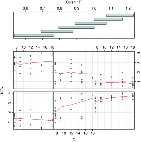
There is a pronounced positive effect of C on NOx only in panel 2 (ethanol 0.7 < E < 0.9 from the shingles in the upper panel), but only slight effects elsewhere (most of the red lines are roughly horizontal). You can estimate the interaction between E and C from the product of the two variables:

CE <- E*C

model2 <- gam(NOx∼s(E)+s(CE))

windows(7,4)

par(mfrow=c(1,2))

 			

plot.gam(model2,residuals=T,pch=16,all.terms=T)

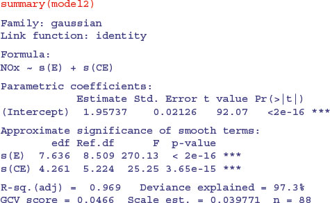
The summary of this GAM shows highly significant terms for both smoothed terms: the effect of ethanol, s(E), on 7.6 estimated degrees of freedom, and the interaction between E and C, s(CE), on 4.3 estimated degrees of freedom. The model explains a highly impressive 97.3% of the deviance in NOx concentration.

18.4 Generalized additive models with binary data

GAMs are particularly valuable with binary response variables (for background, see p. 650). To illustrate the use of gam for modelling binary response data, we return to the example analysed by logistic regression on p. 652. We want to understand how the isolation of an island and its area influence the probability that the island is occupied by our study species.

island <- read.table("c:\\temp\\isolation.txt",header=T)

attach(island)

names(island)

[1] "incidence" "area" "isolation"

In the logistic regression, isolation had a highly significant negative effect on the probability that an island will be occupied by our species (p = 0.004), and area (island size) had a significant positive effect on the likelihood of occupancy (p = 0.019). But we have no a priori reason to believe that the logit of the probability should be linearly related to either of the explanatory variables. We can try using a GAM to fit smoothed functions to the incidence data:

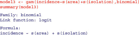
This indicates a highly significant effect of isolation on occupancy (p = 0.006 24) but no effect of area (p = 0.315 22). We plot the model to look at the residuals:

windows(7,4)

par(mfrow=c(1,2))

plot.gam(model3,residuals=T,pch=16)

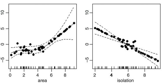
This suggests a strong effect of area, with very little scatter, but only above a threshold of about area = 5. We assess the significance of area by deletion and compare a model containing s(area) + s(isolation) with a model containing s(isolation) alone:

model4 <- gam(incidence∼s(isolation),binomial)

anova(model3,model4,test="Chi")

Analysis of Deviance Table

 	

Model 1: incidence ∼ s(area) + s(isolation)

Model 2: incidence ∼ s(isolation)

 	Resid. Df Resid. Dev		Df Deviance Pr(>Chi)

1		45.571	25.094

2		45.799	29.127 -0.22824		-4.033 0.006461 **

This shows the effect of area to be highly significant (p = 0.006 461), despite the non-significant p value in the summary table of model3. An alternative is to fit area as a parametric term and isolation as a smoothed term:

Again, this shows a significant effect of area on occupancy. The lesson here is that a term can appear to be significant when entered into the model as a parametric term (area has p = 0.019 in model5) but not come close to significance when entered as a smoothed term (s(area) has p = 0.275 in model3). Also, the comparison of model3 and model4 draws attention to the benefits of using deletion with anova in assessing the significance of model terms.

18.5 Three-dimensional graphic output from gam

Here is an example by Simon Wood which shows the kind of three-dimensional graphics that can be obtained from gam using vis.gam when there are two continuous explanatory variables. Note that in this example the smoother works on both variables together, y∼s(x,z):

windows(7,7)

test1 <- function(x,z,sx=0.3,sz=0.4)

 	{(pi**sx*sz)*(1.2*exp(-(x-0.2)^2/sx^2-(z-0.3)^2/sz^2)+

 	0.8*exp(-(x-0.7)^2/sx^2-(z-0.8)^2/sz^2))

 	}

n <- 500

x <- runif(n);z <- runif(n);

y <- test1(x,z)+rnorm(n)*0.1

b4 <- gam(y∼s(x,z))

 			

vis.gam(b4)

Note also that the vertical scale of the graph is the linear predictor, not the response.