Chapter 20
Non-Linear Regression
Sometimes we have a mechanistic model for the relationship between y and x, and we want to estimate the parameters and standard errors of the parameters of a specific non-linear equation from data. Some frequently used non-linear models are shown in Table 20.1. What we mean in this case by ‘non-linear’ is not that the relationship is curved (it was curved in the case of polynomial regressions, but these were linear models), but that the relationship cannot be linearized by transformation of the response variable or the explanatory variable (or both). Here is an example: it shows jaw bone length as a function of age in deer. Theory indicates that the relationship is an asymptotic exponential with three parameters:

Table 20.1 Useful non-linear functions.
| Name | Equation |
| Asymptotic functions | |
| Michaelis–Menten |  |
| 2-parameter asymptotic exponential |  |
| 3-parameter asymptotic exponential |  |
| S-shaped functions | |
| 2-parameter logistic |  |
| 3-parameter logistic |  |
| 4-parameter logistic | 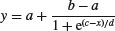 |
| Weibull |  |
| Gompertz |  |
| Humped curves | |
| Ricker curve |  |
| First-order compartment |  |
| Bell-shaped | 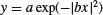 |
| Biexponential |  |
In R, the main difference between linear models and non-linear models is that we have to tell R the exact nature of the equation as part of the model formula when we use non-linear modelling. In place of lm we write nls (this stands for ‘non-linear least squares’). Then, instead of y∼x, we write y∼a-b*exp(-c*x) to spell out the precise non-linear model we want R to fit to the data.
The slightly tedious thing is that R requires us to specify initial guesses for the values of the parameters a, b and c (note, however, that some common non-linear models have ‘self-starting’ versions in R which bypass this step; see p. 728). Let us plot the data to work out sensible starting values. It always helps in cases like this to work out the equation's ‘behaviour at the limits’ – that is to say, to find the values of y when x = 0 and when x = ∞ (p. 258). For x = 0, we have exp(–0) which is 1, and 1 × b = b, so y = a – b. For x = ∞, we have exp(–∞) which is 0, and 0 × b = 0, so y = a. That is to say, the asymptotic value of y is a, and the intercept is a – b.
deer <- read.table("c:\\temp\\jaws.txt",header=T)

attach(deer)

names(deer)
[1] "age" "bone"
plot(age,bone,pch=21,col="purple",bg="green")
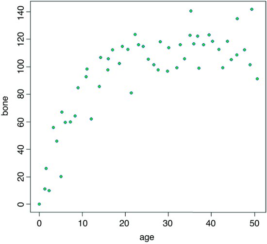
Inspection suggests that a reasonable estimate of the asymptote is a ≈ 120 and intercept ≈ 10, so b = 120 – 10 = 110. Our guess at the value of c is slightly harder. Where the curve is rising most steeply, jaw length is about 40 where age is 5. Rearranging the equation gives

Now that we have the three parameter estimates, we can provide them to R as the starting conditions as part of the nls call like this:
model <- nls(bone∼a-b*exp(-c*age),start=list(a=120,b=110,c=0.064))

summary(model)
Formula: bone ∼ a - b * exp(-c * age)


Parameters:

 Estimate Std. Error t value Pr(>|t|)

a 115.2528		2.9139	39.55 < 2e-16 ***

b 118.6875		7.8925	15.04 < 2e-16 ***

c 0.1235			0.0171	7.22 2.44e-09 ***


Residual standard error: 13.21 on 51 degrees of freedom


Number of iterations to convergence: 5

Achieved convergence tolerance: 2.381e-06
All the parameters appear to be significantly different from zero at p < 0.001. Beware, however. This does not necessarily mean that all the parameters need to be retained in the model. In this case, a = 115.2528 with standard error 2.9139 is clearly not significantly different from b = 118.6875 with standard error 7.8925 (they would need to differ by more than 2 standard errors to be significant). So we should try fitting the simpler two-parameter model
model2 <- nls(bone∼a*(1-exp(-c*age)),start=list(a=120,c=0.064))

anova(model,model2)
Analysis of Variance Table


Model 1: bone ∼ a - b * exp(-c * age)

Model 2: bone ∼ a * (1 - exp(-c * age))


 Res.Df Res.Sum Sq Df Sum Sq F value Pr(>F)

1	51	8897.3

2	52	8929.1 -1 -31.843 0.1825 0.671
Model simplification was clearly justified (p = 0.671), so we accept the two-parameter version, model2, as our minimal adequate model. We finish by plotting the curve through the scatterplot. The age variable needs to go from 0 to 50 in smooth steps:
av <- seq(0,50,0.1)
and we use predict with model2 to generate the predicted bone lengths:
bv <- predict(model2,list(age=av))

lines(av,bv,col="red")

The parameters of this curve are obtained from model2:
summary(model2)
Formula: bone ∼ a * (1 - exp(-c * age))


Parameters:

 Estimate Std. Error t value Pr(>|t|)

a 115.58056		2.84365		40.645 < 2e-16 ***

c	0.11882		0.01233		9.635 3.69e-13 ***


Residual standard error: 13.1 on 52 degrees of freedom


Number of iterations to convergence: 5

Achieved convergence tolerance: 1.356e-06
which we could write as y = 115.58(1 − e–0.1188x) or as y = 115.58(1 – exp(–0.1188x)) according to taste or journal style. If you want to present the standard errors as well as the parameter estimates, you could write: ‘The model y = a (1 – exp(–bx)) had a = 115.58 ± 2.84 (1 standard error) and b = 0.1188 ± 0.0123 (1 standard error, n = 54) and explained 84.87% of the total variation in bone length.’ Note that because there are only two parameters in the minimal adequate model, we have called them a and b (rather than a and c as in the original formulation).
The variation explained needs to be calculated by comparing the residual variation (13.1, above) with the total variation. There are two steps to this. First, work out sse, the variation not explained by the regression. We extract the residual standard error from the model summary (13.1), square it, then multiply by the degrees of freedom (52) to obtain the sum of squares:
sse <- as.vector((summary(model2)[[3]])^2*52)

sse
[1] 8929.143
Second, we work out the total variation in jaw bone length by fitting a null model, estimating only the overall mean, then extract the total sums of squares, sst, from the model summary:
null <- lm(bone∼1)

sst <- as.vector(unlist(summary.aov(null)[[1]][2]))

sst
[1] 59007.99
Now, the percentage variation explained is simply:
100*(sst-sse)/sst
[1] 84.86791
20.1 Comparing Michaelis–Menten and asymptotic exponential
Model choice is always an important issue in curve fitting. We shall compare the fit of the asymptotic exponential (above) with a Michaelis–Menten with parameter values estimated from the same deer jaws data. As to starting values for the parameters, it is clear that a reasonable estimate for the asymptote would be 100 (this is a/b; see p. 264). The curve passes close to the point (5, 40) so we can guess a value of a of 40/5 = 8 and hence b = 8/100 = 0.08. Now use nls to estimate the parameters:
(model3 <- nls(bone∼a*age/(1+b*age),start=list(a=8,b=0.08)))
Nonlinear regression model

 model: bone ∼ a * age/(1 + b * age)

	data: parent.frame()

	 a b

18.725 0.136

 residual sum-of-squares: 9854


Number of iterations to convergence: 7

Achieved convergence tolerance: 1.522e-06
Finally, we can add the line for Michaelis–Menten to the original plot, using predictwith the model name, with a list to allocate av values to age:
yv <- predict(model3, list(age=av))

lines(av,yv,col="blue")

You can see that the asymptotic exponential (red line) tends to get to its asymptote first, and that the Michaelis–Menten (blue line) continues to increase. Model choice, therefore would be enormously important if you intended to use the model for prediction to ages much greater than 50 months.
20.2 Generalized additive models
Sometimes we can see that the relationship between y and x is non-linear but we do not have any theory or any mechanistic model to suggest a particular functional form (mathematical equation) to describe the relationship. In such circumstances, generalized additive models (GAMs) are particularly useful because they fit non-parametric smoothers to the data without requiring us to specify any particular mathematical model to describe the non-linearity (background and more examples are given in Chapter 18).
humped <- read.table("c:\\temp\\hump.txt",header=T)

attach(humped)

names(humped)

[1] "y" "x"

plot(x,y,pch=21,col="brown",bg="orange")

library(mgcv)
The model is specified very simply by showing which explanatory variables (in this case just x) are to be fitted as smoothed functions using the notation y∼s(x):
model <- gam(y∼s(x))
Now we can use predict in the normal way to fit the curve estimated by gam:
xv <- seq(0.5,1.3,0.01)

yv <- predict(model,list(x=xv))

lines(xv,yv)
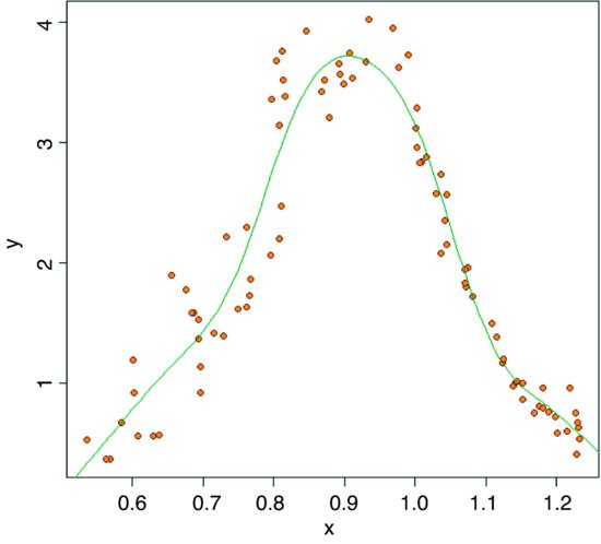
summary(model)
Family: gaussian

Link function: identity


Formula:

y ∼ s(x)


Parametric coefficients:

 Estimate Std. Error t value Pr(>|t|)

(Intercept)	1.95737		0.03446		56.8	<2e-16 ***


Approximate significance of smooth terms:

	edf Ref.df	F p-value

s(x) 7.452 8.403 116.7		<2e-16 ***

R-sq.(adj) = 0.919		Deviance explained = 92.6%

GCV score = 0.1156 Scale est. = 0.1045		n = 88
Fitting the curve uses up 7.452 degrees of freedom (i.e. it is quite expensive) but the resulting fit is excellent and the model explains more than 92.6% of the deviance in y.
20.3 Grouped data for non-linear estimation
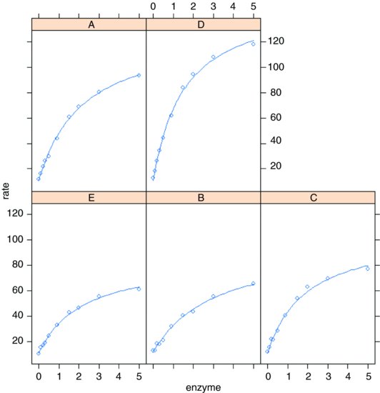
Here is a dataframe containing experimental results on reaction rates as a function of enzyme concentration for five different bacterial strains, with reaction rate measured just once for each strain at each of ten enzyme concentrations. The idea is to fit a family of five Michaelis–Menten functions with parameter values depending on the strain.
reaction <- read.table("c:\\temp\\reaction.txt",header=T)

attach(reaction)

names(reaction)
[1] "strain" "enzyme" "rate"
plot(enzyme,rate,pch=20+as.numeric(strain),bg=1+as.numeric(strain))
Clearly the different strains will require different parameter values, but there is a reasonable hope that the same functional form will describe the response of the reaction rate of each strain to enzyme concentration.
library(nlme)
The function we need is nlsList, which fits the same functional form to a group of subjects (as indicated by the ‘given’ operator |):
model <- nlsList(rate∼c+a*enzyme/(1+b*enzyme)|strain,

 		data=reaction,start=c(a=20,b=0.25,c=10))
Note the use of the groupedData style formula rate∼enzyme|strain.
There is substantial variation from strain to strain in the values of a and b, but we should test whether a model with a common intercept of, say, 11.0 might not fit equally well.
The plotting is made much easier if we convert the dataframe to a groupedData object:
reaction <- groupedData(rate∼enzyme|strain,data=reaction)

plot(reaction)

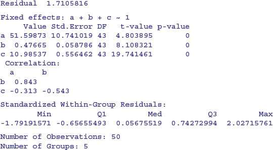
This default plot has just joined the dots, but we want to fit the separate non-linear regressions. To do this we fit a non-linear mixed-effects model with nlme, rather than use nlsList:
model2 <- nlme(rate∼c+a*enzyme/(1+b*enzyme),fixed=a+b+c∼1,

 		random=a+b+c∼1|strain,data=reaction,start=c(a=20,b=0.25,c=10))
Now we can employ the very powerful augPred function to fit the curves to each panel:
plot(augPred(model2))
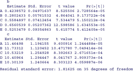
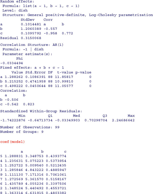
Here is the summary of the non-linear mixed model:
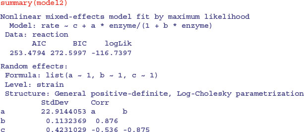
The fixed effects in this model are the means of the parameter values. To see the separate parameter estimates for each strain, use coef:
coef(model2)
	a		b		c

E 34.09244 0.4533741 10.81642

B 28.01211 0.3238606 11.54848

C 49.64062 0.5193966 10.67127

A 53.20342 0.4426117 11.23660

D 93.04507 0.6440231 10.65410
Note that the rows of this table are no longer in alphabetical order but sequenced in the way they appeared in the panel plot (i.e. ranked by their maximum values). The parameter estimates are close to, but not equal to, the values estimated by nlsList (above) as a result of ‘shrinkage’ in the restricted maximum likelihood estimates (see p. 685). The efficiency of the random effects model in terms of degrees of freedom is illustrated by contrasting the numbers of parameters estimated by nlsList (15 = 5 values for each of 3 parameters) and by nlme (7 = 3 parameters plus 4 variances), giving residual degrees of freedom of 35 and 43, respectively.
If you want to draw the fitted lines yourself, then repeat the scatterplot we did earlier:
plot(enzyme,rate,pch=20+as.numeric(strain),bg=1+as.numeric(strain))
and use a loop to extract the three parameters from the coefficients table coef(model) and to copy the colours for the fitted lines:
for(i in 1:5){

yv <- coef(model)[i,3]+coef(model)[i,1]*xv/(1+coef(model)[i,2]*xv)

lines(xv,yv,col=(i+1)) }

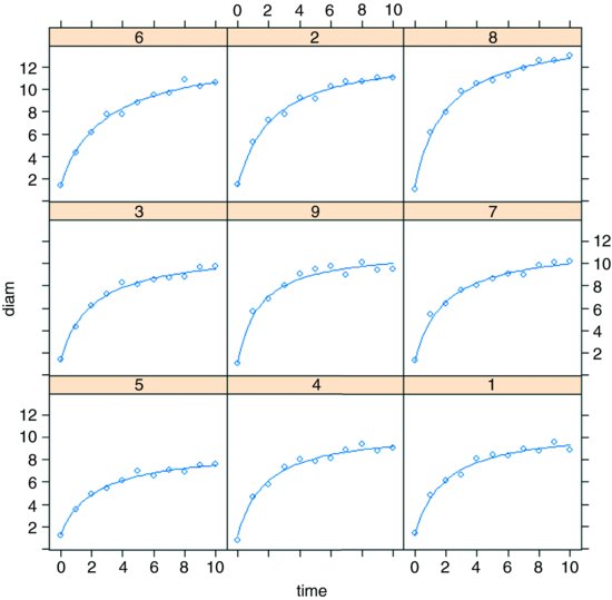
20.4 Non-linear time series models (temporal pseudoreplication)
The previous example was a designed experiment in which there was no pseudoreplication. However, we often want to fit non-linear models to growth curves where there is temporal pseudoreplication across a set of subjects, each providing repeated measures on the response variable. In such a case we shall want to model the temporal autocorrelation.
nl.ts <- read.table("c:\\temp\\nonlinear.txt",header=T)

attach(nl.ts)

names(nl.ts)
[1] "time" "dish" "isolate" "diam"
growth <- groupedData(diam∼time|dish,data=nl.ts)
Here, we model the temporal autocorrelation as first-order autoregessive, corAR1():
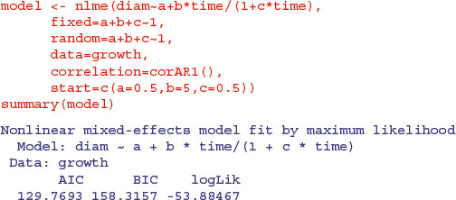
It could not be simpler to plot the family of non-linear models in a panel of scatterplots. We just use augPred like this:
plot(augPred(model))
20.5 Self-starting functions
One of the most likely things to go wrong in non-linear least squares is that the model fails because your initial guesses for the starting parameter values were too far off. The simplest solution is to use one of R's ‘self-starting’ models, which work out the starting values for you automatically. These are the most frequently used self-starting functions:
| SSasymp | asymptotic regression model; |
| SSasympOff | asymptotic regression model with an offset; |
| SSasympOrig | asymptotic regression model through the origin; |
| SSbiexp | biexponential model; |
| SSfol | first-order compartment model; |
| SSfpl | four-parameter logistic model; |
| SSgompertz | Gompertz growth model; |
| SSlogis | logistic model; |
| SSmicmen | Michaelis–Menten model; |
| SSweibull | Weibull growth curve model. |
20.5.1 Self-starting Michaelis–Menten model
In our next example, reaction rate is a function of enzyme concentration; reaction rate increases quickly with concentration at first but asymptotes once the reaction rate is no longer enzyme-limited. R has a self-starting version called SSmicmen, parameterized as

where the two parameters are a (the asymptotic value of y) and b (which is the x value at which half of the maximum response, a/2, is attained). In the field of enzyme kinetics b is called the Michaelis parameter (see p. 264; in R help the two parameters are called Vm and K, respectively).
Here is SSmicmen in action:
data <- read.table("c:\\temp\\mm.txt",header=T)

attach(data)

names(data)
[1] "conc" "rate"
plot(rate∼conc,pch=16)
To fit the non-linear model, just put the name of the response variable (rate) on the left of the tilde ∼ then put SSmicmen(conc,a,b)) on the right of the tilde, with the name of your explanatory variable first in the list of arguments (conc in this case), then your names for the two parameters (a and b, as defined above):
model <- nls(rate∼SSmicmen(conc,a,b))

summary(model)
Formula: rate ∼ SSmicmen(conc, a, b)

Parameters:

 Estimate Std. Error t value Pr(>|t|)

a 2.127e+02	6.947e+00		30.615 3.24e-11 ***

b 6.412e-02	8.281e-03		7.743 1.57e-05 ***


Residual standard error: 10.93 on 10 degrees of freedom


Number of iterations to convergence: 0

Achieved convergence tolerance: 1.93e-06
So the equation is
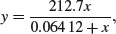
and we can plot it like this:
xv <- seq(0,1.2,.01)

yv <- predict(model,list(conc=xv))

lines(xv,yv,col="blue")
20.5.2 Self-starting asymptotic exponential model
The three-parameter asymptotic exponential is usually written like this:

In R's self-starting version, SSasymp, the parameters are as follows:
- a is the horizontal asymptote on the right-hand side (called Asym in R help);
- b = a – R0 where R0 is the intercept (the response when x is zero);
- c is the rate constant (the log of lrc in R help).
Here is SSasymp applied to the jaws data (p. 209):
deer <- read.table("c:\\temp\\jaws.txt",header=T)

attach(deer)

names(deer)
[1] "age" "bone"
model <- nls(bone∼SSasymp(age,a,b,c))

plot(age,bone,pch=16)

xv <- seq(0,50,0.2)

yv <- predict(model,list(age=xv))

lines(xv,yv)


summary(model)
Formula: bone ∼ SSasymp(age, a, b, c)


Parameters:

 Estimate Std. Error t value Pr(>|t|)

a 115.2527		2.9139	39.553	<2e-16 ***

b	-3.4348		8.1961	-0.419	0.677

c	-2.0915		0.1385	-15.101	<2e-16 ***


Residual standard error: 13.21 on 51 degrees of freedom


Number of iterations to convergence: 0

Achieved convergence tolerance: 2.472e-07
The plot of this fit is on p. 720 along with the simplified model without the non-significant parameter b.
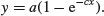
Alternatively, one can use the two-parameter form that passes through the origin, SSasympOrig, which fits the function y = a(1–exp (–bx)). The final form of the asymptotic exponential allows one to specify the function with an offset, d, on the x values, using SSasympOff, which fits the function y = a – b exp (–c(x – d)).
20.5.3 Self-starting logistic
This is one of the most commonly used three-parameter growth models, producing a classic S-shaped curve:
sslogistic <- read.table("c:\\temp\\sslogistic.txt",header=T)

attach(sslogistic)

names(sslogistic)
[1] "density" "concentration"
plot(density∼log(concentration),pch=16,col="green3")
We estimate the three parameters (a, b, c) using the self-starting function SSlogis:
model <- nls(density ∼ SSlogis(log(concentration), a, b, c))
Now draw the fitted line using predict (note the antilog of xv in list):
xv <- seq(-3,3,0.1)

yv <- predict(model,list(concentration=exp(xv)))

lines(xv,yv,col="red")
The fit is excellent, and the parameter values and their standard errors are given by:
summary(model)
Formula: density ∼ SSlogis(log(concentration), a, b, c)


Parameters:

 Estimate Std. Error t value Pr(>|t|)

a	2.34518		0.07815		30.01 2.17e-13 ***

b	1.48309		0.08135		18.23 1.22e-10 ***

c	1.04146		0.03227		32.27 8.51e-14 ***


Residual standard error: 0.01919 on 13 degrees of freedom


Number of iterations to convergence: 0

Achieved convergence tolerance: 3.284e-06
Here a is the asymptotic value, b is the mid-value of x when y is a/2, and c is the scale.
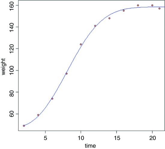
20.5.4 Self-starting four-parameter logistic
This model allows a lower asymptote (the fourth parameter) as well as an upper:
data <- read.table("c:\\temp\\chicks.txt",header=T)

attach(data)

names(data)
[1] "weight" "Time"
model <- nls(weight∼SSfpl(Time, a, b, c, d))

xv <- seq(0,22,.2)

yv <- predict(model,list(Time=xv))

plot(weight∼Time,pch=21,col="red",bg="green4")

lines(xv,yv,col="navy")
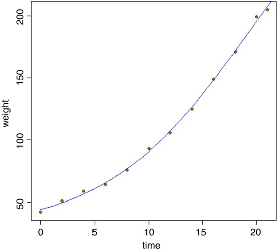
summary(model)
Formula: weight ∼ SSfpl(Time, a, b, c, d)
Parameters:
Estimate Std. Error t value Pr(>|t|)
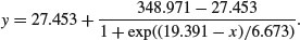
a 27.453 6.601 4.159 0.003169 **
b 348.971 57.899 6.027 0.000314 ***
c 19.391 2.194 8.836 2.12e-05 ***
d 6.673 1.002 6.662 0.000159 ***
Residual standard error: 2.351 on 8 degrees of freedom
Number of iterations to convergence: 0
Achieved convergence tolerance: 3.324e-07
The four-parameter logistic is given by
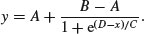
This is the same formula as we used in Chapter 7, but note that C above is 1/c on p. 267. A is the horizontal asymptote on the left (for low values of x), B is the horizontal asymptote on the right (for large values of x), D is the value of x at the point of inflection of the curve (represented by xmid in our model for the chicks data), and C is a numeric scale parameter on the x axis (represented by scal). The parameterized model would be written like this:
20.5.5 Self-starting Weibull growth function
R's parameterization of the Weibull growth function is
Asym-Drop*exp(-exp(lrc)*x^pwr)
where Asym is the horizontal asymptote on the right, Drop is the difference between the asymptote and the intercept (the value of y at x = 0), lrc is the natural logarithm of the rate constant, and pwr is the power to which x is raised.
weights <- read.table("c:\\temp\\weibull.growth.txt",header=T)

attach(weights)

names(weights)
[1] "weight" "time"
model <- nls(weight ∼ SSweibull(time, Asym, Drop, lrc, pwr))

summary(model)
Formula: weight ∼ SSweibull(time, Asym, Drop, lrc, pwr)


Parameters:

 Estimate Std. Error t value Pr(>|t|)

Asym	158.5012		1.1769		134.67 3.28e-13 ***

Drop	110.9971		2.6330		42.16 1.10e-09 ***

lrc	-5.9934		0.3733		-16.05 8.83e-07 ***

pwr	2.6461		0.1613		16.41 7.62e-07 ***


Residual standard error: 2.061 on 7 degrees of freedom


Number of iterations to convergence: 0

Achieved convergence tolerance: 5.702e-06
xt <- seq(2,22,0.1)

yw <- predict(model,list(time=xt))

plot(time,weight,pch=21,col="blue",bg="orange")

lines(xt,yw,col="blue2")
The fit is good, but the model cannot accommodate a drop in y values once the asymptote has been reached (you would need to fit some kind of humped function).
20.5.6 Self-starting first-order compartment function
In the following model, the response is drug concentration in the blood, which is to be plotted as a function of time after the dose was administered. There are three parameters (a, b, c) to be estimated:
foldat <- read.table("c:\\temp\\fol.txt",header=T)

attach(foldat)

names(foldat)
[1] "Wt" "Dose" "Time" "conc"
The model looks like this: the response (y) is conc and the explanatory (x) is Time,

where k = Dose × exp(a + b – c)/(exp(b) – exp(a)) and Dose is a vector of identical values provided in the dataframe (4.02 in this example):
model <- nls(conc∼SSfol(Dose, Time, a, b, c))

summary(model)
Formula: conc ∼ SSfol(Dose, Time, a, b, c)


Parameters:

 Estimate Std. Error t value Pr(>|t|)

a	-2.9196		0.1709	-17.085 1.40e-07 ***

b	0.5752		0.1728	3.328	0.0104 *

c	-3.9159		0.1273	-30.768 1.35e-09 ***


Residual standard error: 0.732 on 8 degrees of freedom


Number of iterations to convergence: 8

Achieved convergence tolerance: 4.907e-06
xv <- seq(0,25,0.1)

yv <- predict(model,list(Time=xv))

plot(conc∼Time,pch=21,col="blue",bg="red")

lines(xv,yv,col="green4")

As you can see, this is a rather poor model for predicting the value of the peak concentration, but a reasonable description of the ascending and declining sections.
20.6 Bootstrapping a family of non-linear regressions
There are two broad applications of bootstrapping to the estimation of parameters in non-linear models:
- Select certain of the data points at random with replacement, so that, for any given model fit, some data points are duplicated and others are left out.
- Fit the model and estimate the residuals, then allocate the residuals at random, adding them to different fitted values in different simulations.
Our next example involves the viscosity data from the MASS library, where sinking time (y = Time) is measured for three different weights (w = Wt) in fluids of nine different viscosities (x = Viscosity):

We need to estimate the two parameters b and c and their standard errors.
library(MASS)

data(stormer)

attach(stormer)
Here are the results of the straightforward non-linear regression:
model <- nls(Time∼b*Viscosity/(Wt-c),start=list(b=29,c=2))

summary(model)
Formula: Time ∼ b * Viscosity/(Wt - c)


Parameters:

 Estimate Std. Error t value Pr(>|t|)

b	29.4013		0.9155	32.114	< 2e-16 ***

c	2.2182		0.6655	3.333	0.00316 **


Residual standard error: 6.268 on 21 degrees of freedom


Number of iterations to convergence: 2

Achieved convergence tolerance: 8.959e-06
plot(Viscosity,Time,pch=16,col=1+as.numeric(factor(Wt)))

xv <- 0:300

yv <- predict(model,list(Wt=20,Viscosity=xv))

lines(xv,yv,col=2)

yv <- predict(model,list(Wt=50,Viscosity=xv))

lines(xv,yv,col=3)

yv <- predict(model,list(Wt=100,Viscosity=xv))

lines(xv,yv,col=4)

Here is a home-made bootstrap which leaves out cases at random. The idea is to sample the indices (subscripts) of the 23 cases at random with replacement:
sample(1:23,replace=T)
[1] 4 4 10 10 12 3 23 22 21 13 9 14 8 5 15 14 21 14 12 3 20 14 19
In this realization cases 1 and 2 were left out, cases 4 and 10 appeared twice, and so on. We call the subscripts ss as follows, and use the subscripts to select values for the response (y) and the two explanatory variables (x1 and x2) like this:
ss <- sample(1:23,replace=T)

y <- Time[ss]

x1 <- Viscosity[ss]

x2 <- Wt[ss]
Now we put this in a loop and fit the model:
model <- nls(y∼b*x1/(x2-c),start=list(b=29,c=2))
one thousand times, storing the coefficients in vectors called bv and cv:
bv <- numeric(1000)

cv <- numeric(1000)

for(i in 1:1000){

ss <- sample(1:23,replace=T)

y <- Time[ss]

x1 <- Viscosity[ss]

x2 <- Wt[ss]

model <- nls(y∼b*x1/(x2-c),start=list(b=29,c=2))

bv[i] <- coef(model)[1]

cv[i] <- coef(model)[2] }
This took 2 seconds for 1000 iterations. The 95% confidence intervals for the two parameters are obtained using the quantile function:
quantile(bv,c(0.025,0.975))
 2.5% 97.5%

27.80559 30.70029
quantile(cv,c(0.025,0.975))
 2.5% 97.5%

0.7798505 3.7625656
Alternatively, you can randomize the locations of the residuals while keeping all the cases in the model for every simulation. We use the built-in functions in the boot package to illustrate this procedure.
library(boot)
The boot package (Canty and Ripley, 2012) allows both parametric and non-parametric resampling. For the non-parametric bootstrap, possible resampling methods are the ordinary bootstrap, the balanced bootstrap, antithetic resampling, and permutation. For non-parametric multi-sample problems stratified resampling is used: this is specified by including a vector of strata in the call to boot. Importance resampling weights may be specified. The function generates a specified number bootstrap replicates (R) of a statistic applied to data. The tricky part is in understanding how to write the statistic function. This is a function which when applied to data returns a vector containing the statistic(s) of interest.
First, we need to calculate the residuals and the fitted values from the nls model we fitted on p. 735:
rs <- resid(model)

fit <- fitted(model)
We make the fit along with the two explanatory variables Viscosity and Wt into a new dataframe called storm that will be used inside the statistic function:
storm <- data.frame(fit,Viscosity,Wt)
Next, we need to write the statistic function to describe the model fitting. We add the randomized residuals to the fitted values, then extract the coefficients from the non-linear model fitted to these new data:
statistic <- function(rs,i){

storm$y <- storm$fit+rs[i]

coef(nls(y∼b*Viscosity/(Wt-c),data=storm,start=coef(model)))}
The two arguments to statistic are the vector of residuals, rs, and the randomized indices, i. Now we can run the boot function over 1000 iterations:
boot.model <- boot(rs,statistic,R=1000)

boot.model
ORDINARY NONPARAMETRIC BOOTSTRAP


Call:

boot(data = rs, statistic = statistic, R = 1000)

Bootstrap Statistics :

	original	bias	std.	error

t1*	29.401294	0.6714883		0.8565776

t2*	2.218247	-0.2528173	0.6177332
The parametric estimates for b (t1) and c (t2) in boot.model are reasonably unbiased, and the bootstrap standard errors are slightly smaller than when we used nls. We get the bootstrapped confidence intervals with the boot.ci function: b is index=1 and c is index=2:
boot.ci(boot.model,index=1)
BOOTSTRAP CONFIDENCE INTERVAL CALCULATIONS

Based on 1000 bootstrap replicates


CALL :

boot.ci(boot.out = boot.model, index = 1)


Intervals :

Level		Normal		Basic

95%	(27.05, 30.41 )		(27.10, 30.42 )


Level		Percentile		BCa

95%		(28.39, 31.70 )		(27.63, 30.39 )

Calculations and Intervals on Original Scale
boot.ci(boot.model,index=2)
BOOTSTRAP CONFIDENCE INTERVAL CALCULATIONS

Based on 1000 bootstrap replicates


CALL :

boot.ci(boot.out = boot.model, index = 2)


Intervals :

Level		Normal		Basic

95%	( 1.260, 3.682 )	( 1.311, 3.735 )


Level		Percentile		BCa

95%	( 0.701, 3.126 )	( 1.250, 3.479 )

Calculations and Intervals on Original Scale
For comparison, here are the parametric confidence intervals from our home-made bootstrap: for b, from 27.80 to 30.70; and for c, from 0.7798 to 3.7625.