Chapter 21
Meta-Analysis
There is a compelling case to be made that analysts should look at the whole body of evidence, rather than trying to understand individual studies in isolation. The systematic review of a body of evidence is known as meta-analysis. The idea is to draw together all of the appropriate studies that have addressed the same question, and calculate an overall effect and an overall measure of uncertainly for that effect. Of course, there are plenty of issues with this, among them the following:
- What do we mean by ‘the same question’?
- What is an appropriate study?
- What makes a study inappropriate ?
- How different can a study be, and still be worth including in the meta-analysis?
- What are the publication biases in the various studies?
- Are the effects fixed or random?
The central idea is to remove as much as possible of the subjectivity that was such a feature of old-fashioned narrative reviews. In an ideal world, we should be able to extract from every published study the exact question addressed, the effect size, the variance of that effect, the replication, and enough detail on the methods used to be confident that the study was comparable with the others that we have already included. Then we simply calculate a weighted average effect size and an appropriate weighted average measure of the unreliability of that overall effect. And that would be it.
If the effect is consistent across experiments, this gives considerable confidence in its generality, and the size of the effect is a useful measure of its importance. On the other hand, if the effect is found to be inconsistent across experiments, then its generality is called into question, and further studies are required to understand why the effect was so variable.
Meta-analysis requires:
- clear rules for the selection of studies;
- clear rules for the omission of studies;
- simple protocols for assigning a statistical weight to each study;
- agreed methods for calculating an appropriate measure of uncertainly for the effect;
- sufficient detail in the Methods section that another analyst would get exactly the same result, and come to exactly the same conclusion, if they were to repeat the analysis using the same group of studies.
A meta-analysis of existing studies would be a useful component of the Introduction of any scientific paper, because it would show what the question was, and why it was interesting. Likewise, the Discussion section would benefit from a meta-analysis of existing studies, by showing what the current study means and where it fits into existing knowledge.
It is very important that biases are investigated and reported. We can never know how many experiments were carried out but never published. We can make an educated guess, but we can never know for certain. It is highly likely that proportionately more studies go unpublished if they failed to find a significant effect. It is possible (but regrettable) that more manuscripts were rejected during the refereeing process if they reported non-significant effects. All of the effect sizes from all of the relevant studies must be included in the analysis (not just the most pleasing ones). The variation in the effect sizes might be due to sampling effects alone, or there may be genuine differences in the effects reported by different studies.
The idea is to calculate an effect size and a variance for each study. The summary of the meta-analysis is then just a weighted average of these effect sizes. More precise studies are given more weight than less precise ones in calculating the summary effect.
21.1 Effect size
Meta-analysis can work with a variety of kinds of effects. The simplest effects would be arithmetic means. Or we might choose to work with the differences between control and treatment means. Alternatively, we could use the scaled difference (the raw difference between the treatment and control means, divided by the pooled standard deviation). In other circumstances, we might look at the ratio between the two means. This is called a response ratio, R, and it is often used in cases where the response variable is a continuous measurement (like yield in an agricultural trial). R is the mean value for the treatment divided by the mean value of the control. Often in such cases, the effect size we analyse is the logarithm of this ratio, because this is symmetric above and below zero, and is hence more likely to have normal errors.
For count data, proportion data and binary data (dead or alive, recovered or ill) we cannot use linear models, because we shall have non-constant variance and non-normal errors (see Chapter 13). In such cases, we might use the risk ratio, the odds ratio or the risk difference. For studies reporting correlation coefficients we might do a meta-analysis of the correlation coefficients. In any event, the sampling distribution of the effect size should be known, so that variances and confidence intervals can be computed.
21.2 Weights
More precise studies should be given higher weights. Typically this means that studies with higher replication get higher weights, but the details depend on our assumptions about the distribution of the true effects. Many meta-analyses use the inverse of the variances as weights (the less variable a study, the more weight is given to that effect).
21.3 Fixed versus random effects
If you can convince yourself that there is a single true effect size (for instance, if many studies are trying to estimate the same physical constant) then the fixed-effect model is appropriate. It is much more likely in practice, however, that the effect being estimated varies with the context (e.g. with location, genetics or environmental conditions). In such cases, it is appropriate to do a random-effects meta-analysis. In this case, the measured effects are assumed to represent a random sample from a distribution of effect sizes.
21.3.1 Fixed-effect meta-analysis of scaled differences
This example comes from Borenstein et al. (2009) and concerns six studies each with a treatment and a control group, with replication varying from 40 to 200 across studies:
data <- read.table("c:\\temp\\metadata.txt",header=T)

attach(data)

head(data)
 study	meanT	sdT		nT	meanC	sdC		nC

1	A	94		22		60	92		20		60

2	B	98		21		65	92		22		65

3	C	98		28		40	88		26		40

4	D	94		19		200	82		17		200

5	E	98		21		50	88		22		45

6	F	96		21		85	92		22		85
The effect size for each study in this case is going to be the scaled difference between the treatment and control means:
d <- meanT-meanC

d
[1] 0.0951303 0.2789943 0.3701166 0.6656402 0.4655727 0.1859962
Work out the pooled within-study standard deviation, using the formulae in Table 21.1. Note the use of round brackets to print the answer, avoiding typing swithin again:
Table 21.1 Calculations for a fixed-effects meta-analysis. The individual effects (Y) have variances (V) reflecting sampling error alone. Study weights (W) are the inverse of the study variances. The assumption is that there is a common overall fixed effect, of which M is our best estimate. Nomenclature follows Borenstein et al. (2009).
| Term | Formula |
| Weight |  |
| Weighted mean summary effect |  |
| Variance of the summary effect |  |
| Standard error of the summary effect |  |
| Lower limit on the summary effect | M−1.96 SEM |
| Upper limit on the summary effect | M+1.96 SEM |
| Test statistic |  |
(swithin <- sqrt(((nT-1)*sdT^2+(nC-1)*sdC^2)/(nT+nC-2)))
[1] 21.02380 21.50581 27.01851 18.02776 21.47892 21.50581
Scale the difference between the means by the pooled within-study standard deviation – this will be the effect size in our meta-analysis:
(d <- d/swithin)
[1] 0.0951303 0.2789943 0.3701166 0.6656402 0.4655727 0.1859962
Calculate the variance of the scaled difference:
(Vd <- (nC+nT)/(nC*nT) + d^2/(2*(nC+nT)))
[1] 0.03337104 0.03106861 0.05085616 0.01055385 0.04336305 0.02363116
Compute Hedges' g (g) and its variance (Vg) of the bias-corrected mean difference:
(J <- 1-3/(4*(nC+nT-2)-1))
[1] 0.9936306 0.9941292 0.9903537 0.9981144 0.9919137 0.9955291
(g <- J*d)
[1] 0.09452437 0.27735640 0.36654635 0.66438510 0.46180798 0.18516464
(Vg <- J^2*Vd)
[1] 0.03294729 0.03070488 0.04987975 0.01051408 0.04266460 0.02342033
Confidence intervals (int) for the scaled differences (lower limit ll, and upper limit, ul) are computed next:
(int <- 1.96*sqrt(Vg))
[1] 0.3557672 0.3434470 0.4377420 0.2009749 0.4048461 0.2999525
(ll <- d-int)
[1] -0.26063689 -0.06445270 -0.06762538 0.46466536 0.06072666 -0.11395631
(ul <- d+int)
[1] 0.4508975 0.6224414 0.8078586 0.8666151 0.8704188 0.4859488
As a flourish, we compute the total samples for each experiment (ns) to use in making the square symbols in the forest plot:
(ns <- nT+nC)
[1] 120 130 80 400 95 170
Now for the summary effect. First, work out the weights (the reciprocals of the variances)
(W <- 1/Vg)
[1] 30.35151 32.56811 20.04822 95.11053 23.43864 42.69795
Now calculate the sum of the products of the weight and the effects:
(WY <- W*g)
[1] 2.868958 9.032975 7.348601 63.190019 10.824149 7.906151
Here are the calculations so far – effect size, variance within, weight, and weight by effect:
data.frame(d,Vd,W,WY)
		d		Vd			W		WY

1 0.0951303	0.03337104	30.35151	2.868958

2 0.2789943	0.03106861	32.56811	9.032975

3 0.3701166	0.05085616	20.04822	7.348601

4 0.6656402	0.01055385	95.11053	63.190019

5 0.4655727	0.04336305	23.43864	10.824149

6 0.1859962	0.02363116	42.69795	7.906151
The summary effect is the sum of the products WY divided by the sum of the weights W:
(M <- sum(WY)/sum(W))
[1] 0.4142697
The variance of the summary effect is just the reciprocal of the sum of the weights:
(VM <- 1/sum(W))
[1] 0.004094753
Finally, we want the standard error of the mean effect which is the square root of VM, and the value of the test statistic, z:
(SEM <- sqrt(VM))
[1] 0.06399026
(z <- M/SEM)
[1] 6.473949
(ci <- 1.96*SEM)
[1] 0.1254209
The forest plot needs to show the six studies (labelled A–F) and their unreliability estimates, with the summary effect and its unreliability estimate shown as a diamond at the bottom (in a different colour for emphasis):
plot(c(-1,1),c(0,8),type="n",xlab="",yaxt="n",ylab="")

points(d,8-(1:6),pch=15,cex=10*ns/sum(ns))

for (i in 1:7) lines(c(ll[i],ul[i]),c(8-i,8-i))

polygon(c(M-ci,M,M+ci,M),c(1,1.1,1,0.9),col="red")

abline(v=0,lty=2)

text(rep(-0.7,7),1:7,c("summary effect","F","E","D","C","B","A"))
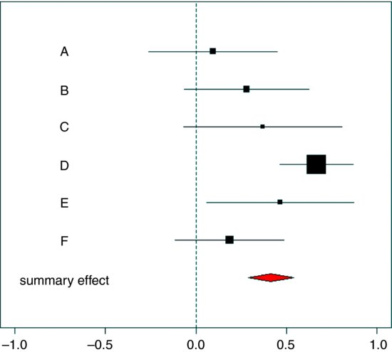
It is important to note that so-called ‘vote counting’ gets the wrong answer: only two significant results (D and E) out of six suggests non-significance overall. Not so. The summary effect is highly significant, and the lower bound of the red diamond comes nowhere near the vertical dashed line showing no effect. The sizes of the squares show the fraction of all replicates (across the six studies) that come from each study (the relative weights = ns/sum(ns)).
As an exercise, you might like to convert the above code into a simple general function that will work with any number of studies. It should take six vectors as its arguments (mean, standard deviation and sample size for treatment, then the same for control, for each of the studies in a meta-analysis).
If you are doing a meta-analysis in earnest, you are likely to use the meta package (Schwarzer, 2012). Here is the last example, repeated using metacont (this stands for ‘meta-analysis for continuous variables’):
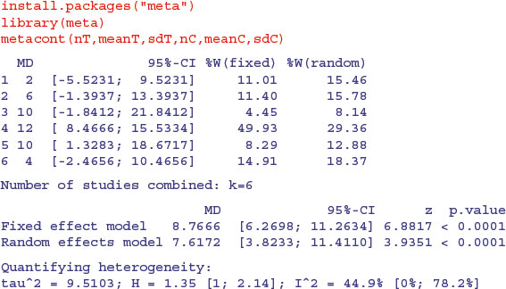
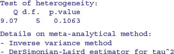
There was no significant heterogeneity across the treatments (p = 0.1063). Here is its forest plot:
forest(metacont(nT,meanT,sdT,nC,meanC,sdC))

This output shows both the fixed-effect and the random-effect analysis of these data: in this case, the interpretation is the same under both models, but this need not be so. Note that the mean effect size is smaller and the significance lower under the random-effects model.
Table 21.2 Calculations for a random effects meta-analysis. The individual effects (Y) have variances (V) reflecting sampling error alone as in Table 21.1. The total variance V* now has two components: the within study variance (V) and the between study variance T2 (tau squared). The method of moments (DerSimonian and Laird method) calculates T2 from three quantities: Q (a corrected weighted sum of squares of the individual effects), C (a corrected sum of weights) and d.f. (degrees of freedom, one less than the number of studies k), where W and Y are as defined in Table 21.1. If all the studies had the same sample variance  and were based on the same sample size n, then the standard error of the summary effect would be
 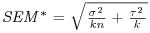 . Nomenclature follows Borenstein et al. (2009).
| Term | Formula |
| Q | 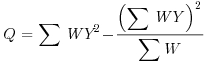 |
| C | 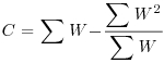 |
| Degrees of freedom | d.f. = k – 1 |
| Between-study variance (tau squared) | 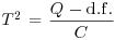 |
| Total variance |  |
| Weight |  |
| Weighted mean summary effect | 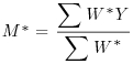 |
| Variance of the summary effect | 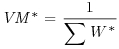 |
| Standard error of the summary effect |  |
21.3.2 Random effects with a scaled mean difference
We repeat the analysis using a random effects model, using the formulae in Table 21.2. We start by computing the components Q, d.f. and C, from which we shall calculate the between study variance, tau-squared.
WY2 <- W*g^2

W2 <- W^2

Q <- sum(WY2)-(sum(WY)^2/sum(W))

Q
[1] 12.00325
df <- 6-1

df
[1] 5
C <- sum(W)-(sum(W2)/sum(W))

C
[1] 187.6978
T2 <- (Q-df)/C

T2
[1] 0.03731131
So the DerSimonian and Laird estimate of between-study variance, tau-squared, is 0.0373. For the random-effects estimate of the summary effect, we need to allow for shrinkage (see p. 685). The weights are the reciprocals of the total variance (within Vg plus between T2):
Wstar <- 1/(Vg+T2)

Wstar
[1] 14.23313 14.70238 11.46907 20.90940 12.50377 16.46588
Mstar <- sum(Wstar*g)/sum(Wstar)

Mstar
[1] 0.3582294
Vstar <- 1/sum(Wstar)

Vstar
[1] 0.01107621
SEMstar <- sqrt(Vstar)

SEMstar
[1] 0.1052436
LLstar <- Mstar-1.96*SEMstar

ULstar <- Mstar+1.96*SEMstar
LLstar
[1] 0.1519521

ULstar

[1] 0.5645068
Zstar <- Mstar/SEMstar

Zstar
[1] 3.403813
Because of shrinkage, the random effects estimate of the mean effect (Mstar = 0.358) is smaller than the fixed effects estimate (M = 0.414), as illustrated in the forest plot from metacont (above).
21.4 Random-effects meta-analysis of binary data
Next we demonstrate a random effects meta-analysis on count data. Instead of a difference between means, the effect in this analysis is the log-odds ratio, based on proportion data from six different studies (A–F) each with two treatments (control, C, and treated, T). The count data are the number of deaths (success) and number of survivors (failure; the data come from Borenstein et al., 2009):

We should get a quick overview of the effects before starting the calculations. In the treatment group, the total number of successes was 83 and the total number of failures was 607, so the odds of success were
sum(successT)/sum(failureT)
[1] 0.1367381
In the control group, the total number of successes was 154 and the total number of failures was 536, so the odds of success were
sum(successC)/sum(failureC)
[1] 0.2873134
Now a rough and ready estimate of the overall effect size is given by the odds ratio, which is the treatment odds divided by control odds:
(sum(successT)/sum(failureT))/(sum(successC)/sum(failureC))
[1] 0.4759195
indicating that treatment has reduced the effect by roughly 50% (47.6%) taking the six studies together. The meta-analysis proceeds as follows, using the formulae in Table 21.2.
First, use the raw count data to compute a vector of odds ratios (or), one for each study (the number of successes divided by number of failures for the treated group, divided by the same quantity for the control group):
(or <- successT*failureC/(failureT*successC))
[1] 0.6933962 0.7500000 0.6810207 0.2666667 0.6590909 0.8526077
The response variable in this kind of meta-analysis is the logarithm of the odds ratio (lor)
(lor <- log(or))
[1] -0.3661537 -0.2876821 -0.3841625 -1.3217558 -0.4168938 -0.1594557
The variance of the log-odds ratio for each of the six studies is the sum of the reciprocals of the four counts of success and failure:
(vlor <- 1/successT + 1/failureT + 1/successC + 1/failureC)
[1] 0.18510942 0.28958333 0.15560511 0.05829167 0.28164185 0.15974031
As usual in meta-analysis, the weight given to each study is the reciprocal of its variance:
(W <- 1/vlor)
[1] 5.402210 3.453237 6.426524 17.155111 3.550609 6.260160
Note the very high weight given to study 4 (17.16) because of its large sample size.
In order to carry out the meta-analysis using the random-effects model, we need to calculate a set of products and sums of products (Borenstein et al., 2009): WY is the vector of products of the weights times the effect sizes, and WY2 is the vector of products of the weights times the squares of the effect sizes:
WY <- W*lor

WY2 <- W*lor^2
The fundamental difference with the random-effects model is that we compute a variance in the true effect (traditionally denoted by tau squared,  ) as well as the separate, per-study variances. For this we use the DerSimonian and Laird (1986) method
  , where the quantities Q, d.f. and C are computed as follows:
Q <- sum(WY2)-(sum(WY)^2/sum(W))

df <- length(nC)-1

C <- sum(W)-(sum(W^2)/sum(W))

T2 <- (Q-df)/C
Here is a summary of the results so far:
(res <- data.frame(sum(WY),sum(WY2),Q,df,C,T2))
 sum.WY.		sum.WY2.		Q df		C		T2

1 -30.59362	32.7054		10.55115 5 32.10525 0.1729048
The subsequent random-effects analysis is based on the assumption that the variance for each study is the sum of the within-study variance (vlor) and the between-study variance (T2). The new weights to be given to each study (Wstar) are therefore calculated like this:
(Wstar <- 1/(T2+vlor))
[1] 2.793185 2.162218 3.044048 4.325325 2.199994 3.006207
Note that although D is still the most highly weighted of the studies, the relative size of its weight is substantially reduced in the random effects model (down from 17.16 to 4.33). To calculate the summary effect size we need the sum of the weights and the sum of the products of the weights times the effect sizes:
(Mstar <- sum(Wstar*lor)/sum(Wstar))
[1] -0.5662959
This is the summary of the log-odds ratio across the six studies. We back-transform to the odds ratio by taking the antilog of Mstar:
exp(Mstar)
[1] 0.5676241
Note that the summary effect is considerably larger than the rough preliminary calculation we made earlier (0.4759, above). The unreliability estimates associated with the summary effect are calculated like this (V = variance, SE = standard error, ll = lower limit, ul = upper limit):
VMstar <- 1/sum(Wstar)

SEMstar <- sqrt(VMstar)

llMstar <- Mstar-1.96*SEMstar

ulMstar <- Mstar+1.96*SEMstar

Z <- Mstar/SEMstar

p <- 2*(1-pnorm(-Z))
Here is a summary of the random-effects model output:
(res2 <- data.frame(Mstar,SEMstar,llMstar,ulMstar,Z,p))
	Mstar	SEMstar		llMstar		ulMstar		Z		p

1 -0.5662959 0.2388344		-1.034411		-0.09818041 -2.371081 0.01773612
The forest plot looks like this:
ll<-lor-1.96*vlor

ul<-lor+1.96*vlor
plot(c(-2,0.3),c(0,8),type="n",xlab="",yaxt="n",ylab="")

points(lor,8-(1:6),pch=15,cex=10*Wstar/sum(Wstar))

for (i in 1:7) lines(c(ll[i],ul[i]),c(8-i,8-i))

polygon(c(llMstar,Mstar,ulMstar,Mstar),c(1,1.2,1,0.8),col="red")

abline(v=0,lty=2)

text(rep(-1.8,7),1:7,c("summary effect","F","E","D","C","B","A"))

The summary effect is highly significant (note the log-odds scale), with zero effect marked as the vertical dashed line at 0. As before, note that vote counting would have led to the wrong conclusion (only two significant studies out of six).