Chapter 22

Bayesian Statistics

Instead of asking ‘what do my data show?’, the Bayesian analyst asks ‘how do my data alter our view of the world?'. It may not sound like much, but it is a fundamental change of outlook. The idea is that the results of the new study are assessed in the light of the existing data, to establish an updated assessment of parameter values and their uncertainties. There are now two models rather than one. There is a model for what we know already: this is called the prior. Then there is a model that we fit to our data: this is the likelihood. The two models combine to give us an estimate of the posterior. We use the posterior distribution to make statistical inferences. Under its Bayesian interpretation, probability measures our confidence that something is true.

When the new study is small, and existing knowledge is extensive, then we should not expect our work to make much difference to overall understanding. For instance, if we studied 150 subjects and found that age at death was not affected by their smoking habits, we would be ill advised to conclude that this result had great generality. This is because we know from studies of many thousands of subjects over many decades that smoking leads to a reduction of about 14 years in mean age at death. Small studies can be highly informative, of course, especially when they are original and address important questions. But the larger and better designed the new study, the more that study should be capable of altering our prior knowledge, and if the study is big enough and sufficiently well conducted, then it could turn prior expectation on its head. A Bayesian analysis works in three steps:

• using all the currently available information to create a full probability model;
• forming a posterior inference by conditioning the full probability model on the new data;
• criticizing the fit of the model to the data and evaluating the predictions it makes.

You should read Bayesian Data Analysis by Gelman et al. (2004) for background, examples and computational methods on each of these steps.

One of the strengths of the Bayesian approach is that it does not rely on two of the most peculiar aspects of the frequentist approach. Beginners often think that:

• if I reject the null hypothesis at the 5% level, then there is a 5% chance that the null hypothesis is true;
• if I establish a 95% confidence interval for the value of a parameter, then the value of the parameter lies within these bounds with probability 0.95.

Of course, both these assertions are wrong, but they are wrong in ways that are genuinely hard for beginners to understand. In the first case, the p value (say 0.05) means that a test statistic as large, or larger, than the one we observed, is expected to occur by chance alone with probability 0.05 when the null hypothesis is true. True, it is a measure of the plausibility of the null hypothesis, but it is not the probability that it is true, because we calculated the test statistic on the basis that the null hypothesis really was true. In the second case, we are asked to do an imaginary experiment in which we repeat our data collection exercise many times. The confidence interval indicates the distribution of these hypothetical repeated estimates of the parameter. It does not mean that the probability that our estimated parameter value lies outside these bounds is 0.05. But this is precisely what a Bayesian credible interval means.

Bayesians talk naturally about the probability of hypotheses:

• the unconditional probability of an hypothesis (its prior probability);
• the conditional probability, given some new evidence (its posterior probability).

The advantages of Bayesian analysis include the following:

• All sources of variation can be modelled (fixed effects, random effects, measurement error, etc.).
• All unknowns are treated as random variables.
• Confidence intervals are intuitive. The highest posterior density (HPD, also known as the credible interval) refers to the observed data on which the distribution of the parameter is conditioned – this is a much more intuitive concept than the conventional 95% confidence interval, which is based on some hypothetical replications of the sample.
• Explanatory variables known to be of substantive importance are included in the model even if they appear not to be statistically significant (e.g. density dependence in population models).
• Models can be as complex as necessary to describe the question in hand.
• Interpretation of complex models is much more straightforward.
• The uncertainly associated with missing values (so-called multiple imputation) is dealt with more satisfactorily.
• Multiple comparisons are dealt with intuitively, including comparisons of structurally different models.
• The very term ‘hypothesis testing’ dictates that it should be the hypothesis that is tested, given the data, not the other way around.

However, Bayesian analysis has a number of disadvantages:

• You need to know much more maths and statistics to do it competently.
• The solution to realistically complicated models can only be achieved through iterative simulation, drawing random samples from the posterior distribution.
• There are many ways of carrying out these simulations and it is not obvious in advance which method will be most effective.
• The choice of priors can be both controversial and consequential, especially with small sample sizes.
• Simulation is not exact, and it may not be obvious that you have the best possible model for the posterior.

To illustrate what I mean by needing to be better at statistics, consider these simple questions. What, precisely does ‘knowing nothing’ mean in terms of choosing between different priors? Should we assume that different parameters in the prior are independent of one another? What number of new observations do you reckon your prior information is worth ? How do I ensure that priors are conjugate? I think you will see what I mean.

Analytical solutions to simple Bayesian problems are relatively straightforward, so long as we stick to well-known distributions like the normal or the Poisson and use conjugate priors. But for realistically complicated models, it is essential to resort to numerical simulation to work out the parameter values involved in quantifying the posterior distribution.

It is not so much the priors that represent the principal motivation for using Bayesian models these days, but rather the potential to include all of the important sources of variation in a straightforward way. This has revolutionized statistical modelling in many fields. Estimating parameter values and their credible intervals by numerical simulation from the posterior distribution represents a quantum step in dealing with the most complicated models, including models with a high ratio of parameters to data points, and hierarchical models with complex spatial or temporal structure.

22.1 Background

We need to revise some simple probability theory. Let us define E as an event, and H as an hypothesis (a model) about the likelihood of E. The probability of an event E, given the hypothesis H, is written as P(E|H), which is read ‘the probability of E given H'. Some straightforward rules apply:

• for all E and all H;
• P(H|H) = 1 for all H;
• 

The first just says that you cannot have negative probabilities. The second just says that the hypothesis needs to encompass all possible outcomes. The third is the subtle one. It says that given independent events E and F, then the probability of getting E and F given the hypothesis (the right-hand side), is the product of the probability of F given the hypothesis, times the probability of E given both F and H. Take the example of twins. They can derive from splitting of a single fertilized egg (monozygotic twins), or from two separate fertilizations of different eggs (dizygotic twins). Not all monozygotic twins look ‘identical’, and some dizygotic individuals can look very alike. This means that you cannot reliably tell monozygotic from dizygotic twins just by looking at them. But there is a reliable way of estimating the proportions of monozygotic and dizygotic twins in the population. The key fact is that while dizygotic twins can be 2 boys or 2 girls or 1 boy and 1 girl, monozygotic twins are always of the same sex. So if B is the event of a twin being a boy, and G is the event of a twin being a girl, then there are three outcomes for any batch of twins: BB, GG or BG. Let us define the second event as either monozygotic (M) or dizygotic (D). The probabilities for the dizygotic twins are easy:

The probabilities for monozygotic twins include the fact that P(BG|M) is impossible:

We want to know P(M). Using what we have learned about conditional probability, we can write down the probability of getting two girls if we know P(M) and P(D).

Half of all monozygotic twins will be GG but only one quarter of dizygotic twins will be GG:

from which we can extract P(M) by multiplying through the bracket by , subtracting from , then subtracting from both sides to leave

so the answer is P(M) = 4P(GG)−1. In a town where 45% of twins are girl–girl, the proportion of twins that are monozygotic is 100 × ((4 × 0.45) – 1) = 80%.

22.2 A continuous response variable

Suppose that our data are X and our model contains the parameters θ. We might ask what is the probability of observing our data given that the model is true? This is called the frequentist approach to maximum likelihood (see p. 390):

Alternatively, because we are usually a lot more certain about our data than we are about the truth of our model, we might ask what is the likelihood of our model, given the data:

These two quantities are different ways of expressing the same idea, but they embody a fundamentally different approach. You need to think about this last paragraph until the penny drops.

The fundamental part of Bayesian statistics is that the posterior distribution is proportional to the product of the prior and the likelihood:

This tells us how to modify our existing beliefs in the light of the newly available data. Note the proportionality: we can multiply the likelihood by any constant without affecting the posterior, but we need our posterior probability distribution to integrate to 1.

22.3 Normal prior and normal likelihood

The simplest Bayesian calculations are in cases where both the prior and the likelihood are normal. Assume that we have a single unknown parameter for which our prior is expressed in terms of a normal distribution for which we know both the mean () and the variance (). We have collected new data X with sample mean μ and known variance .

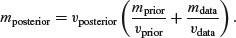
The traditional way to measure precision is by the inverse of the variance (i.e. posterior precision = prior precision+data precision). We start by getting the overall estimate of the posterior variance: this is the reciprocal of the sum of the reciprocals of the prior variance and the sample variance:

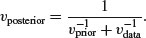
The posterior mean is the weighted mean of the prior and the data, using the inverse variances as the weights:

Now, of course, there are many assumptions here. The most important is that the two variances and the prior mean are known without error, and that the unknown parameter is normally distributed. These assumptions are all relaxed in more advanced Bayesian models.

Let us take a simple example, just to illustrate the concept of shrinkage. Suppose that Smith was the first to estimate the productivity of this particular kind of grassland, and she found a mean of 500 units per unit area with a standard deviation of 25. Our new data give a mean of 420 with a standard deviation of 10. If we use Smith's findings as our prior, we get a posterior variance, v, of roughly 86 like this:

(v <- 1/(1/25^2+1/10^2))

[1] 86.2069

The posterior mean is given by

(v*(500/25^2 + 420/10^2))

[1] 431.0345

So the prior was N(500, 252), the likelihood from the new data was N(420, 102) and the posterior was N(431, 92). The new mean is closer to the likelihood than to the prior, and the standard deviation is substantially lower.

Jones, working a decade later than Smith, found a mean of 400 with a standard deviation of 20. How much difference would it have made if we had taken Jones rather than Smith for our estimate of the prior? Now the posterior variance would be

(v2 <- 1/(1/20^2+1/10^2))

[1] 80

and the new posterior mean would be

(v2*(400/20^2 + 420/10^2))

[1] 416

The posterior variance is roughly the same as before, but the posterior mean is slightly lower: N(416, 92) compared to N(431, 92). So our choice of priors does matter, and the smaller our new sample, the more that choice matters. With three studies, we might have done a meta-analysis (see Chapter 21).

22.4 Priors

Your prior beliefs can be specified as a point estimate (a single value) or as a distribution (many values, each with a different probability density). My prior for tossing this fair coin is a point estimate: the probability of heads is . My prior for the yield of a new crop is 10% higher than the yield of the conventional crop (μ = 1.1), but with a similar variance (): this could be expressed as a normal prior .

22.4.1 Conjugate priors

The likelihood function is and the prior is . If the posterior density

is in the same family of distributions as the prior, then the class of prior distributions is said to form a conjugate family. The prior is called a conjugate prior for the likelihood. In most cases, this makes the maths much more straightforward, since the posterior has the same algebraic form as the prior. A classic example comes from the case where the response variable follows a binomial distribution with a single parameter, π, the probability of success in a single trial. The choice of a prior for π is best if , where B is a beta distribution, because the family of beta distributions is conjugate to a binomial likelihood. Roughly speaking, you can choose α and β so that α+β represents the number of observations that you reckon your prior information is worth, while the mean of the beta distribution is equal to (Lee, 2012). The conjugate prior distribution for a response variable that has a Poisson likelihood (e.g. count data) is the gamma distribution. And so on. All the likelihood functions belonging to the exponential family have conjugate priors that are also in the exponential family (see Chapter 27).

Conjugate priors are useful if you are aiming for an analytical solution, but not essential if you intend to investigate your posterior distribution numerically. It is impossibly slow to calculate the probability associated with every combination of circumstances and every value of every parameter of the current model. We need a cleverer way of homing in on the right answer. It is in these cases that Markov chain Monte Carlo (MCMC) methods come into their own.

22.5 Bayesian statistics for realistically complicated models

Model choice is a very important part of Bayesian data analysis. Not only do we have to select a deterministic structure for the likelihood (which explanatory variables to include, and how to relate them to the response variable and to one another), but also specify a joint probability distribution for all the observable and unobservable quantities involved in the problem. This is known as the full probability model. Then, given the data, we need to compute the appropriate posterior distribution: this is the conditional probability distribution of all the unobserved quantities, given the observed data. Finally, we must subject the model to criticism: how good is the fit to the data, are the conclusions reasonable, and how sensitive is the interpretation to the assumptions that are embodied in the model choice? We cannot expect to be able to do these things analytically. The most popular methods for solving these issues numerically involve simulations known collectively as Markov chain Monte Carlo methods.

The Monte Carlo part of the name refers to random draws (the gambling part). The Markov chain part of the name refers to a series of events where what happens next depends only on current status (and not on any memory of historical status). The idea is step-by-step to better approximate the target posterior distribution (hill climbing is a useful analogy). Samples are drawn sequentially, with the distribution of the sample draws depending only on the last sample drawn, such that the approximate distributions are improved at every step. With time, the simulation converges on the target posterior distribution (Gelman et al., 2004).

The Metropolis algorithm is a kind of random walk that uses an acceptance/rejection rule to converge on a specified target distribution. It uses what is called a jumping distribution that either stays where it is or moves to a new place, with the probability of movement to a new place depending on the ratio of probability densities between the new place and the existing place. It always accepts steps that increase the density, but occasionally accepts downward steps. This ensures that the solution does not get stuck on small, local maxima that are some way distant from the global maximum. The Metropolis–Hastings algorithm differs in two ways: the jumping rules no longer need to be symmetric, and ratio of densities is modified to account for this asymmetry. The Gibbs sampling algorithm generates an instance from the distribution of each variable in turn, conditional on the current values of the other variables.

22.6 Practical considerations

MCMC modelling involves two important practical considerations: the burn-in period and thinning. By throwing away the early values from the simulation, the effects of the initial conditions will have died away, leaving a better estimate of the posterior distribution. The burn-in period (from which the results are discarded) is often set to half of the chain.

Because the hill-climbing process is based on a Markov chain, successive values of the parameters show strong serial correlations, so successive values typically give little extra information about the shape of the posterior distribution. You might choose to take one point in every hundred or so, to reduce the serial correlation. This is the thinning rate.

22.7 Writing BUGS models

BUGS stands for ‘Bayesian inference Using Gibbs Sampling’ (Lunn et al., 2009). You can read about the history of BUGS at the OpenBUGS website http://www.openbugs.info/w/.

The trick is to learn how to express your particular model in BUGS code. The code looks superficially like R, but it is fundamentally different. You do not type the code into R, but you write it in an editor, and save it as an ASCII file outside of R. The name of the file containing your BUGS model is provided as an argument to the MCMC function inside R. You can find lots of clear examples of the way that different kinds of models are expressed in BUGS code on the website for WinBUGS (Spiegelhalter et al., 2003) at http://www.mrc-bsu.cam.ac.uk/bugs/winbugs under the headings ‘Volume 1’, ‘Volume 2’ and ‘Volume 3’ at the bottom of ‘Introduction to WinBUGS’ on the home page. You should spend time browsing through these examples to find the one closest to the problem you are trying to solve, then edit the code to tailor it to your specific requirements. Three examples are described in detail below (a simple regression, a study with temporal pseudoreplication, and an experiment involving proportion data with overdispersion).

22.8 Packages in R for carrying out Bayesian analysis

There is a huge amount of information, and a great many computing resources for Bayesian analysis available on the CRAN website. This is summarized in the Bayesian Inference Task View written by Jong Hee Park (University of Chicago, USA), Andrew D. Martin (Washington University, St. Louis, MO, USA), and Kevin M. Quinn (University of California, Berkeley, USA); see http://cran.r-project.org/web/views/Bayesian.html. The Task View subdivides the packages under five headings:

• Bayesian packages for general model fitting;
• Bayesian packages for specific models or methods;
• post-estimation tools (like coda);
• packages for learning Bayesian statistics;
• packages that link R to other sampling engines (like R2jags, R2WinBUGS, R2OpenBUGS).

Applied researchers interested in Bayesian statistics are increasingly attracted to R because of the ease of which one can code algorithms to sample from posterior distributions as well as the significant number of packages contributed to CRAN. In particular, there are several choices for MCMC sampling. For many years the most popular of these was WinBUGS (Spiegelhalter et al., 2003), and this can still be run from R using the function R2WinBUGS. This is not used here because WinBUGS does not run on a Mac, and the software is no longer being developed. The final manifestation of WinBUGS, frozen at version 1.4.3, is still perfectly functional, but it has been replaced as an evolving framework by OpenBUGS. This means that the main choice is between OpenBUGS and JAGS. I have chosen to illustrate this chapter using JAGS because people who use it a lot speak very highly of it, and because, unlike WinBUGS, it runs on Macs as well as PC and Linux. It may well be that OpenBUGS will become the standard in future, and if it does, it will be simple to switch from JAGS.

22.9 Installing JAGS on your computer

JAGS stands for ‘Just Another Gibbs Sampler’ (Plummer, 2012). It is a program for analysis of Bayesian hierarchical models using MCMC simulation. It is very like BUGS in spirit and language, and was written with three aims in mind:

• to have a cross-platform engine for the BUGS language;
• to be extensible, allowing users to write their own functions, distributions and samplers;
• to be a platform for experimentation with ideas in Bayesian modelling.

JAGS is licensed under the GNU General Public License. First, you need to install JAGS on your machine. You do this by visiting http://mcmc-jags.sourceforge.net/. Click on ‘files page’ under Downloads, then after “Looking for the latest version?” click on Download JAGS. Then run the program and chose all the default options that are offered.

22.10 Running JAGS in R

The next thing you have to do is install the R2jags package that allows R to communicate with JAGS and vice versa. Inside R, while running R as administrator, install the package in the usual way:

install.packages("R2jags")

Now you are ready to start Bayesian modelling. The first thing to appreciate is that you do most of the hard work outside R. You have to use the BUGS language to write down your model of the likelihood and the priors, incorporating all of the important details about hierarchical structure, pseudoreplication, and so forth. Having sketched out the model, you write it in a text editor and save it as an ASCII file (*.txt file). Only now do you go into R to start the modelling. This is the sequence of events:

• Use read.table to enter your data into a dataframe in the familiar way.
• attach the dataframe and make a list of the variable names that need to be passed into the BUGS code.
• Work out the initial conditions (if any) that you want to specify.
• Load the jags package using library(jags).
• Run the JAGS model by specifying the name of the list of variables, the initial conditions (optional), the path and name of the file where the BUGS code is to be found, and the number of Markov chains that you want to run (a popular choice is three).

With any luck the JAGS model will run, and its progress is indicated by a slowly moving horizontal bar. Once the model has finished, you can inspect the parameter estimates and their uncertainty measures, and create various plots.

22.11 MCMC for a simple linear regression

In our example (analysed in detail as a linear model on p. 450) the response variable is growth and the continuous explanatory variable is the concentration of tannin in the diet. We start by reading the data into R:

data2 <- read.table("d:\\temp\\regression.txt",header=T)

attach(data2)

head(data2)

 growth tannin

1	12	0

2	10	1

3	8	2

4	11	3	

5	6	4

6	7	5

Here is a reminder of the output of the simple linear regression for comparison with the JAGS output in due course:

summary(lm(growth∼tannin))

		Estimate Std.	Error	t	value Pr(>|t|)

(Intercept) 11.7556		1.0408	11.295	9.54e-06 ***

tannin	-1.2167		0.2186	-5.565	0.000846 ***

The intercept is 11.7556 (±1.0408) and the slope is –1.2167 (±0.2186).

Outside R, write the BUGS model and save it in a text file. This is the part that you will find difficult at first. The model contains the information on the structure of the model relating the response variable to the explanatory variables (growth = a + b * tannin), the nature of the priors (normal), and the assumed distributions (again, normal). You need to specify the number of rows in the dataframe (N = 9), the formula for the likelihood, and the probability density functions from which the priors and the likelihood are to be selected. This is what the contents of the ASCII file look like:

model {

for (i in 1:N) {

growth[i] ∼ dnorm(mu[i], tau)

mu[i] <- a + b * tannin[i]

}

a ∼ dnorm(0.0, 1.0E-4)

b ∼ dnorm(0.0, 1.0E-4)

sigma <- 1.0/sqrt(tau)

tau ∼ dgamma(1.0E-3, 1.0E-3)

}

The model contains a mixture of deterministic and stochastic elements. The deterministic components are indicated by ‘gets’ <- symbols: mu[i] <- a + b * tannin[i] and sigma <- 1.0/sqrt(tau). The stochastic components are indicated by a tilde (∼): the likelihood growth[i] ∼ dnorm(mu[i], tau), the prior for the intercept a ∼ dnorm(0.0, 1.0E-4), the uninformative prior for the slope b ∼ dnorm(0.0, 1.0E-4), while tau is sampled from a gamma distribution tau ∼ dgamma(1.0E-3, 1.0E-3). The code is saved to a file called c:\\temp\\regression.bugs.txt in this example. Now go back into R.

We need to open the library to connect our R session with the JAGS program:

library(R2jags)

You need to tell the jags function several important things:

• the names of the variables containing the data to which the model will be fitted;
• initial values for the parameters (you can omit this, and let JAGS figure them out);
• the names of the parameters to save for interpretation and inference;
• the name of the path and the ASCII file where the code for the model is to be found;
• the number of chains you want to simulate;
• the number of iterations per chain (by default, the burn-in is half this number).

Tell jags the names of the variables containing the data:

data.jags <- list("growth", "tannin", "N")

Finally, run the jags function to produce the model:

model <- jags(data=data.jags, parameters.to.save=c("a", "b", "tau"),

 n.iter=100000, model.file="C:/temp/regression.bugs.txt", n.chains=3)

Compiling model graph

 Resolving undeclared variables

 Allocating nodes

 Graph Size: 46

We inspect the model output like this:

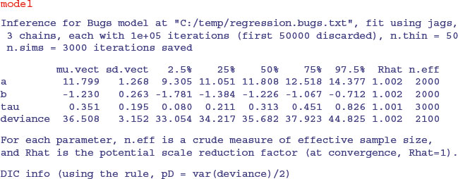
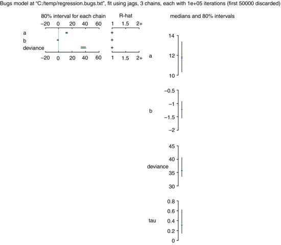
As you can see, the parameter estimates are very close to those obtained by the linear model (intercept = 11.799 ± 1.268 rather than 11.7556 ±1.0408; slope = –1.230 ±0.263 rather than –1.2167 ±0.2186). The unreliability estimates are slightly greater than in the linear model, and the deviance is substantially greater (36.51 rather than 20.07), but the interpretation is unaffected. A plot of the jags model object produces strip diagrams with credible interval bars for the parameters, the deviance and tau, with the results from the different chains in different colours:

plot(model)

You can obtain some attractive graphical output using functions from the coda package:

model.mcmc <- as.mcmc(model)

densityplot(model.mcmc)

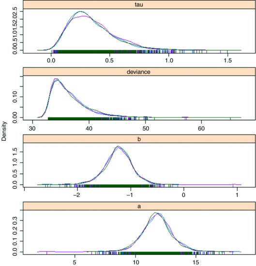
This shows each of the three chains in a different colour, and gives a clear visual impression of the unreliability of the estimates of the two model parameters (intercept a and slope b) and tau (the reciprocal of the error variance). Note the strong positive skew in the distribution of deviance.

22.12 MCMC for a model with temporal pseudoreplication

The root growth of N individuals was measured over T time periods. The temporal pseudoreplication is built into the BUGS model in the form of nested loops (time j within individual i). Mean size (mu) is assumed to be a linear function of time (x) with intercept alpha and slope beta. The data are plotted on p. 695, where they are analysed with a linear mixed effects model:

data <- read.table("d:\\temp\\fertilizer.txt",header=T)

attach(data)

head(data)

	root		week	plant	fertilizer

1	1.3		2	ID1		added

2	3.5		4	ID1		added

3	7.0		6	ID1		added

4	8.1		8	ID1		added

5	10.0		10	ID1		added

6	2.0		2	ID2		added

Write the BUGS model and save it to an ASCII file called c:\\temp\\bayes.lme.txt:

model

{

for( i in 1 : N ) {

for( j in 1 : T ) {

Y[i , j] ∼ dnorm(mu[i , j],tau.c)

mu[i , j] <- alpha[i] + beta[i] * (x[j])

}

alpha[i] ∼ dnorm(alpha.c,alpha.tau)

beta[i] ∼ dnorm(beta.c,beta.tau)

}

tau.c ∼ dgamma(0.001,0.001)

sigma <- 1 / sqrt(tau.c)

alpha.c ∼ dnorm(0.0,1.0E-6)

alpha.tau ∼ dgamma(0.001,0.001)

beta.c ∼ dnorm(0.0,1.0E-6)

beta.tau ∼ dgamma(0.001,0.001)

alpha0 <- 0

}

The issues in this example concern the shape of the data. The response (root length) needs to be a matrix Y with the individuals as the rows (not a single vector as root is at present):

Y <- root

dim(Y) <- c(5,12)

Y <- t(Y)

The explanatory variable (week) needs to be a vector x of length T = 5 (not length 60 as at present):

x <- week[1:5]

We need to provide jags with the names of the variables containing the data:

data.jags <- list("Y", "x", "N","T")

Finally, we can run the jags model like this:

model <- jags(data=data.jags,

	parameters.to.save=c("alpha", "beta", "tau.c","alpha.c",

	"alpha.tau","beta.c","beta.tau"), n.iter=100000,

	model.file="C:/temp/bayes.lme.txt", n.chains=3)

This may take a few seconds to execute, but then we can investigate the posterior estimates of the parameters and their associated uncertainty measures:

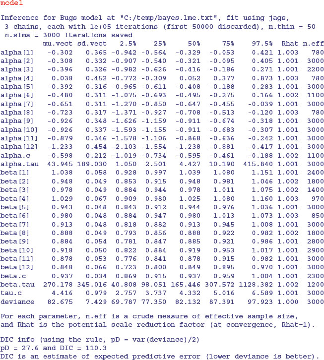
As you can see, there is convincing evidence of non-linearity here, because several of the individuals (7–12) have intercepts significantly less than zero. There is also significant variation in the slopes (from 1.038 down to 0.848, with standard deviation less than 0.067).

22.13 MCMC for a model with binomial errors

We analysed this model for the percentage germination of seeds from a factorial experiment involving two genotypes of Orobanche and two extracts, as a GLM with quasi-binomial errors on p. 636. Here are the data: the response, count, is the number germinating out of an initial sample of seeds (i.e. 10 germinated out of 39 seeds in the first case):

data <- read.table("c:\\temp\\germination.txt",header=T)

attach(data)

head(data)

 count sample Orobanche extract

1	10	39	a75		bean

2	23	62	a75		bean

3	23	81	a75		bean

4	26	51	a75		bean

5	17	39	a75		bean

6	5	6	a75		cucumber

Write the BUGS model and save it in as ASCII file called c:\\temp\\bayes.glm.txt:

model

{

for( i in 1 : N ) {

r[i] ∼ dbin(p[i],n[i])

b[i] ∼ dnorm(0.0,tau)

logit(p[i]) <- alpha0 + alpha1 * x1[i] + alpha2 * x2[i] +

alpha12 * x1[i] * x2[i] + b[i]

}

alpha0 ∼ dnorm(0.0,1.0E-6)

alpha1 ∼ dnorm(0.0,1.0E-6)

alpha2 ∼ dnorm(0.0,1.0E-6)

alpha12 ∼ dnorm(0.0,1.0E-6)

tau ∼ dgamma(0.001,0.001)

sigma <- 1 / sqrt(tau)

}

The deterministic part of the model shows the prediction of logit(p) as a function of the factorial combination of extract and genotype with two main effects (x1 and x2) and one interaction term (the product x1 by x2). The stochastic terms involve the number of germinating seedlings drawn from a binomial distribution (dbin) with parameters p and n, r[i] ∼ dbin(p[i],n[i]), the residuals on the logit scale with normal errors b[i] ∼ dnorm(0.0,tau), with independent, non-informative priors for the intercept, the two main effects and the interaction term (alpha0, alpha1, alpha2 and alpha12), with tau selected from a gamma distribution.

The data we need to provide to the model are:

N <- 21

n <- sample

r <- count

x1 <- Orobanche

x2 <- extract

data.jags <- list("r", "n", "x1", "x2", "N")

Now run the model:

model <- jags(data=data.jags,

parameters.to.save=c("alpha0", "alpha1","alpha2","alpha12","tau"),

n.iter=100000, model.file="C:/temp/bayes.glm.txt", n.chains=3)

To inspect the output, write:

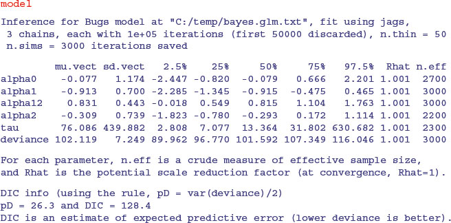
As we saw with the GLM with overdispersion, the interaction term (alpha12) falls short of significance and should be removed. Rewriting the simpler model is left as an exercise.