Chapter 23
Tree Models
Tree models are computationally intensive methods that are used in situations where there are many explanatory variables and we would like guidance about which of them to include in the model. Often there are so many explanatory variables that we simply could not test them all, even if we wanted to invest the huge amount of time that would be necessary to complete such a complicated multiple regression exercise. Tree models are particularly good at tasks that might in the past have been regarded as the realm of multivariate statistics (e.g. classification problems). The great virtues of tree models are as follows:
- They are very simple.
- They are excellent for initial data inspection.
- They give a very clear picture of the structure of the data.
- They provide a highly intuitive insight into the kinds of interactions between variables.
It is best to begin by looking at a tree model in action, before thinking about how it works. Here is an air pollution example that we might want to analyze as a multiple regression. We begin by using tree, then illustrate the more modern function rpart (which stands for ‘recursive partitioning’)
install.packages("tree")

library(tree)

Pollute <- read.table("c:\\temp\\Pollute.txt",header=T)

attach(Pollute)

names(Pollute)
[1] "Pollution" "Temp" "Industry" "Population" "Wind"

[6] "Rain" "Wet.days"
model <- tree(Pollute)

plot(model)

text(model)
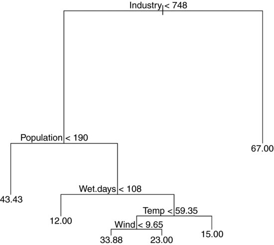
You follow a path from the top of the tree (called, in defiance of gravity, the root) and proceed to one of the terminal nodes (called a leaf) by following a succession of rules (called splits). The numbers at the tips of the leaves are the mean values in that subset of the data (mean SO2 concentration in this case). The details are explained below.
23.1 Background
The model is fitted using binary recursive partitioning, whereby the data are successively split along coordinate axes of the explanatory variables so that, at any node, the split which maximally distinguishes the response variable in the left and the right branches is selected. Splitting continues until nodes are pure or the data are too sparse (fewer than six cases, by default; see Breiman et al., 1984).
Each explanatory variable is assessed in turn, and the variable explaining the greatest amount of the deviance in y is selected. Deviance is calculated on the basis of a threshold in the explanatory variable; this threshold produces two mean values for the response (one mean above the threshold, the other below the threshold).
low <- (Industry<748)

tapply(Pollution,low,mean)
	FALSE	TRUE

67.00000		24.91667
plot(Industry,Pollution,pch=16)

abline(v=748,lty=2)

lines(c(0,748),c(24.92,24.92))

lines(c(748,max(Industry)),c(67,67))
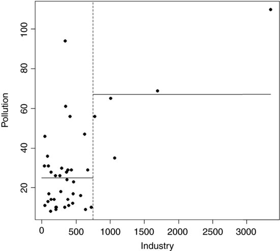
The procedure works like this. For a given explanatory variable (say, Industry above):
- Select a threshold value of the explanatory variable (the vertical dotted line at Industry = 748).
- Calculate the mean value of the response variable above and below this threshold (the two horizontal solid lines).
- Use the two means to calculate the deviance (as with SSE, see p. 500).
- Go through all possible values of the threshold (values on the x axis).
- Look to see which value of the threshold gives the lowest deviance.
- Split the data into high and low subsets on the basis of the threshold for this variable.
- Repeat the whole procedure on each subset of the data on either side of the threshold.
- Keep going until no further reduction in deviance is obtained, or there are too few data points to merit further subdivision (e.g. the right-hand side of the Industry split, above, is too sparse to allow further subdivision).
The deviance is defined as
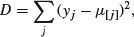
where  is the mean of all the values of the response variable assigned to node j and this sum of squares is add up over all the nodes. The value of any split is defined as the reduction in this residual sum of squares. The probability model used in R is that the values of the response variable are normally distributed within each leaf of the tree with mean μi and variance σ2. Note that because this assumption applies to the terminal nodes, the interior nodes represent a mixture of different normal distributions, so the deviance is only appropriate at the terminal nodes (i.e. for the leaves).
If the twigs of the tree are categorical (i.e. levels of a factor like names of particular species) then we have a classification tree. On the other hand, if the terminal nodes of the tree are predicted values of a continuous variable, then we have a regression tree.
The key questions are these:
- Which variables to use for the division.
- How best to achieve the splits for each selected variable.
It is important to understand that tree models have a tendency to over-interpret the data: for instance, the occasional ‘ups’ in a generally negative correlation probably do not mean anything substantial.
23.2 Regression trees
In this case the response variable is a continuous measurement, but the explanatory variables can be any mix of continuous and categorical variables. You can think of regression trees as analogous to multiple regression models. The difference is that a regression tree works by forward selection of variables, whereas we have been used to carrying out regression analysis by deletion (backward selection).
For our air pollution example, the regression tree is fitted by stating that the continuous response variable Pollution is to be estimated as a function of all of the explanatory variables in the dataframe called Pollute by use of the ‘tilde dot’ notation like this:
model <- tree(Pollution ∼ . , Pollute)
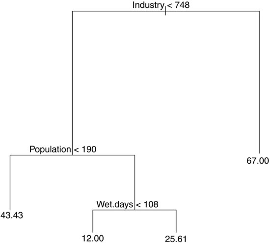
For a regression tree, the print method produces the following kind of output:
print(model)
node), split, n, deviance, yval

	* denotes terminal node


1) root 41 22040 30.05

 2) Industry < 748 36 11260 24.92

	4) Population < 190 7 4096 43.43 *

	5) Population > 190 29 4187 20.45

		10) Wet.days < 108 11 96 12.00 *

		11) Wet.days > 108 18 2826 25.61

		 22) Temp < 59.35 13 1895 29.69

			44) Wind < 9.65 8 1213 33.88 *

			45) Wind > 9.65 5 318 23.00 *

		 23) Temp > 59.35 5 152 15.00 *

 3) Industry > 748 5 3002 67.00 *
The terminal nodes (the leaves) are denoted by * (there are six of them). The node number is on the left, labelled by the variable on which the split at that node was made. Next comes the ‘split criterion’ which shows the threshold value of the variable that was used to create the split. The number of cases going into the split (or into the terminal node) comes next. The penultimate figure is the deviance at that node. Notice how the deviance goes down as non-terminal nodes are split. In the root, based on all n = 41 data points, the deviance is SSY (see p. 499) and the y value is the overall mean for Pollution. The last figure on the right is the mean value of the response variable within that node or at that that leaf. The highest mean pollution (67.00) was in node 3 and the lowest (12.00) was in node 10.
Note how the nodes are nested: within node 2, for example, node 4 is terminal but node 5 is not; within node 5 node 10 is terminal but node 11 is not; within node 11, node 23 is terminal but node 22 is not, and so on.
Tree models lend themselves to circumspect and critical analysis of complex dataframes. In the present example, the aim is to understand the causes of variation in air pollution levels from case to case. The interpretation of the regression tree would proceed something like this:
- The five most extreme cases of Industry stand out (mean = 67.00) and need to be considered separately.
- For the rest, Population is the most important variable but, interestingly, it is low populations that are associated with the highest levels of pollution (mean = 43.43). Ask yourself which might be cause, and which might be effect.
- For high levels of population (greater than 190), the number of wet days is a key determinant of pollution; the places with the fewest wet days (less than 108 per year) have the lowest pollution levels of anywhere in the dataframe (mean = 12.00).
- For those places with more than 108 wet days, it is temperature that is most important in explaining variation in pollution levels; the warmest places have the lowest air pollution levels (mean = 15.00).
- For the cooler places with lots of wet days, it is wind speed that matters: the windier places are less polluted than the still places.
This kind of complex and contingent explanation is much easier to see, and to understand, in tree models than in the output of a multiple regression.
23.3 Using rpart to fit tree models
The newer function rpart differs from tree in the way it handles surrogate variables, but for the most part, it follows Breiman et al. (1984) quite closely. The name of the function stands for ‘recursive partitioning’. We can compare the outputs of rpart (left) and tree (right) for the pollution data:
Pollute<-read.table("c:\\temp\\Pollute.txt",header=T)

attach(Pollute)

names(Pollute)

par(mfrow=c(1,2))


library(rpart)

model<-rpart(Pollution∼.,data=Pollute)

plot(model)

text(model)


library(tree)

model<-tree(Pollute)

plot(model)

text(model)
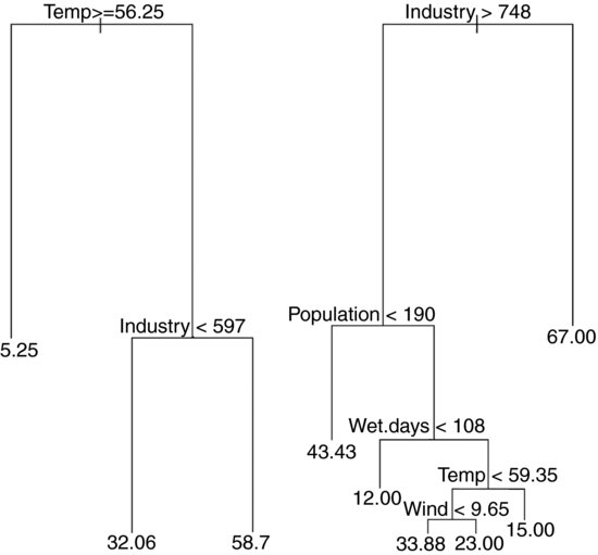
The new function rpart is much better at anticipating the results of model simplification, because it carries out analysis of variance with the two-level factors associated with each split. Thus, for temperature and industry
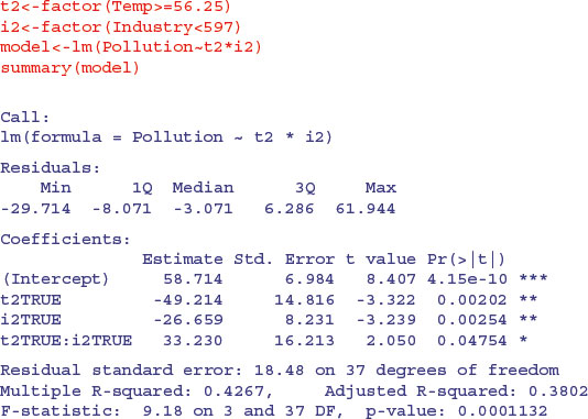
it produces a significant interaction (shown by the split on right branch the tree diagram) and this model does not allow the inclusion of any other significant terms. If population is added, it is marginally significant, but the original interaction between temperature and industry disappears.
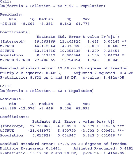
Note that the regression model with t2 and Population has a lower residual standard error (17.95 on 38 d.f.) than the ANOVA from the model suggested by rpart (18.48 on 37 d.f.).
In summary, I prefer the tree function for data inspection, because it shows more detail about the potential interaction structure in the dataframe. On the other hand, rpart is much better at anticipating the results of model simplification. I recommend you use them both, and get the benefit of two perspectives on your data set before embarking on the time-consuming business of carrying out a comprehensive multiple regression exercise.
23.4 Tree models as regressions
To see how a tree model works when there is a single, continuous response variable, it is useful to compare the output with a simple linear regression. Take the relationship between mileage and weight in the car.test.frame data:
car.test.frame <- read.table("c:\\temp\\car.test.frame.txt",header=T)

attach(car.test.frame)

names(car.test.frame)
[1] "Price" "Country" "Reliability" "Mileage"

[5] "Type" "Weight" "Disp." "HP"
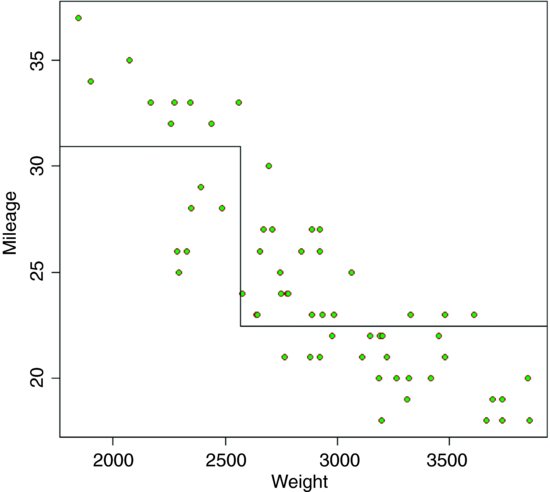
plot(Weight,Mileage,pch=21,col="brown",bg="green")
The heavier cars do fewer miles per gallon, but there is a lot of scatter. The tree model starts by finding the weight that splits the mileage data in a way that explains the maximum deviance. This weight turns out to be 2567.5.
a <- mean(Mileage[Weight<2567.5])

b <- mean(Mileage[Weight>=2567.5])

lines(c(1500,2567.5,2567.5,4000),c(a,a,b,b))
The next thing the tree model does is to work out the threshold weight that would best split the mileage data for the lighter cars: this turns out to be 2280. It then works out the threshold split for the heavier cars: this turns out to be 3087.5. And so the process goes on, until there are too few cars in each split to justify continuation (five or fewer by default). To see the full regression tree as a function plot we can use the predict function with the regression tree object car.model like this:
car.model <- tree(Mileage∼Weight)

wt <- seq(1500,4000)

y <- predict(car.model,list(Weight=wt))

plot(Weight,Mileage,pch=21,col="brown",bg="green")

lines(wt,y)
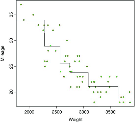
You would not normally do this, of course (and you could not do it with more than two explanatory variables) but it is a good way of showing how tree models work with a continuous response variable.
23.5 Model simplification
Model simplification in regression trees is based on a cost–complexity measure. This reflects the trade-off between fit and explanatory power (a model with a perfect fit would have as many parameters as there were data points, and would consequently have no explanatory power at all). We return to the air pollution example analysed earlier, where we fitted the tree model object called model.
Regression trees can be over-elaborate and can respond to random features of the data (the so-called training set). To deal with this, R contains a set of procedures to prune trees on the basis of the cost–complexity measure. The function prune.tree determines a nested sequence of sub-trees of the supplied tree by recursively ‘snipping’ off the least important splits, based upon the cost–complexity measure. The prune.tree function returns an object of class tree.sequence, which contains the following components:
prune.tree(model)
$size

[1] 6 5 4 3 2 1
This shows the number of terminal nodes in each tree in the cost–complexity pruning sequence: the most complex model had six terminal nodes (see above)
$dev:

[1] 8876.589 9240.484 10019.992 11284.887 14262.750 22037.902
This is the total deviance of each tree in the cost–complexity pruning sequence.
$k:

[1] -Inf 363.8942 779.5085 1264.8946 2977.8633 7775.1524
It is the value of the cost–complexity pruning parameter of each tree in the sequence. If determined algorithmically (as here, k is not specified as an input), its first value defaults to –∞, its lowest possible bound.
plot(prune.tree(model))
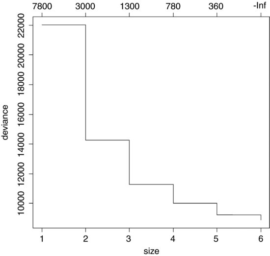
This shows the way that deviance declines as complexity is increased. The total deviance is 22 037.902 (size = 1), and this is reduced as the complexity of the tree increases up to six nodes. An alternative is to specify the number of nodes to which you want the tree to be pruned; this uses the "best=" option. Suppose we want the best tree with four nodes:
model2 <- prune.tree(model,best=4)

plot(model2)

text(model2)
In printed form, this is:
print(model2)
node), split, n, deviance, yval

 * denotes terminal node


 1) root 41 22040 30.05

	2) Industry < 748 36 11260 24.92

	 4) Population < 190 7 4096 43.43 *

	 5) Population > 190 29 4187 20.45

		10) Wet.days < 108 11	96 12.00 *

		11) Wet.days > 108 18 2826 25.61 *

	3) Industry > 748 5 3002 67.00 *
It is straightforward to remove parts of trees, or to select parts of trees, using subscripts. For example, a negative subscript [–3] leaves off everything above node 3, while a positive subscript [3] selects only that part of the tree above node 3.
23.6 Classification trees with categorical explanatory variables
Tree models are a superb tool for helping to write efficient and effective taxonomic keys.
Suppose that all of our explanatory variables are categorical, and that we want to use tree models to write a dichotomous key. There is only one entry for each species, so we want the twigs of the tree to be the individual rows of the dataframe (i.e. we want to fit a tree perfectly to the data). To do this we need to specify two extra arguments: minsize = 2 and mindev = 0. In practice, it is better to specify a very small value for the minimum deviance (say, 10–6) rather than zero (see below).
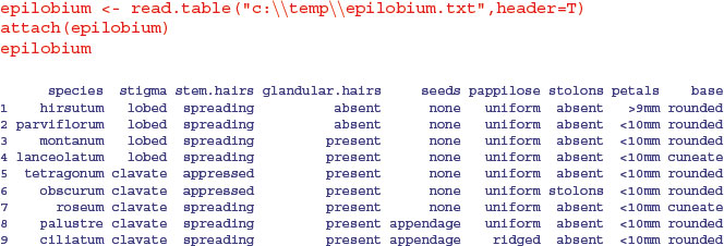
The following example relates to the nine lowland British species in the genus Epilobium (Onagraceae). We have eight categorical explanatory variables and we want to find the optimal dichotomous key. The dataframe looks like this:
Producing the key could not be easier:
model <- tree(species ∼ .,epilobium,mindev=1e-6,minsize=2)

plot(model)

text(model,cex=0.7)
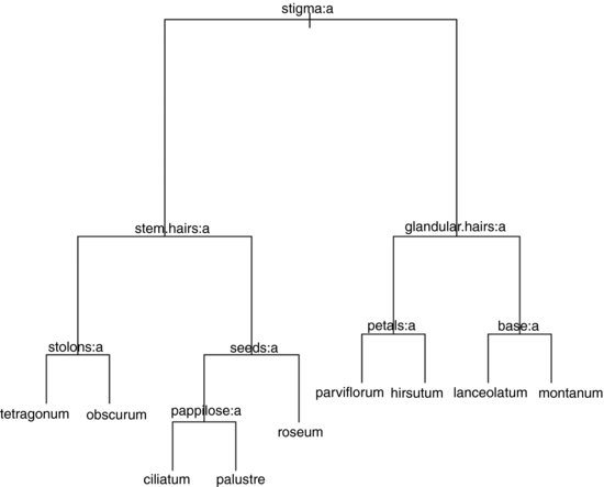
Here is the tree written as a dichotomous key:
| 1. Stigma entire and club-shaped | 2 |
| 1. Stigma four lobed | 6 |
| 2. Stem hairs all appressed | 3 |
| 2. At least some stem hairs spreading | 4 |
| 3. Glandular hairs present on hypanthium | E. obscurum |
| 3. No glandular hairs on hypanthium | E. tetragonum |
| 4. Seeds with a terminal appendage | 5 |
| 4. Seeds without terminal appendage | E. roseum |
| 5. Surface of seed with longitudinal papillose ridges | E. ciliatum |
| 5. Surface of seed uniformly papillose | E. palustre |
| 6. At least some spreading hairs non-glandular | 7 |
| 6. Spreading hairs all glandular | 8 |
| 7. Petals large (>9 mm) | E. hirsutum |
| 7. Petals small (<10 mm) | E. parviflorum |
| 8. Leaf base cuneate | E. lanceolatum |
| 8. Leaf base rounded | E. montanum |
The computer has produced a working key to a difficult group of plants. The result stands as testimony to the power and usefulness of tree models. The same principle underlies good key-writing as is used in tree models: find the characters that explain most of the variation, and use these to split the cases into roughly equal-sized groups at each dichotomy.
23.7 Classification trees for replicated data
In this next example from plant taxonomy, the response variable is a four-level categorical variable called Taxon (it is a label expressed as Roman numerals I to IV). The aim is to use the measurements from the seven morphological explanatory variables to construct the best key to separate these four taxa (the ‘best’ key is the one with the lowest error rate – the key that misclassifies the smallest possible number of cases).
taxonomy <- read.table("c:\\temp\\taxonomy.txt",header=T)

attach(taxonomy)

names(taxonomy)
[1] "Taxon" "Petals" "Internode" "Sepal" "Bract" "Petiole"

[7] "Leaf" "Fruit"
Using the tree model for classification could not be simpler:
model1 <- tree(Taxon∼., taxonomy)
We begin by looking at the plot of the tree:
plot(model1)

text(model1)

With only a small degree of rounding on the suggested break points, the tree model suggests a simple (and for these 120 plants, completely error-free) key for distinguishing the four taxa:
| 1. Sepal length >4.0 | Taxon IV |
| 1. Sepal length ≤4.0 | 2. |
| 2. Leaf width >2.0 | Taxon III |
| 2. Leaf width ≤2.0 | 3. |
| 3. Petiole length <10 | Taxon II |
| 3. Petiole length ≥10 | Taxon I |
The summary option for classification trees produces the following:
summary(model1)
Classification tree:

tree (formula = Taxon ∼ ., data = taxonomy)

Variables actually used in tree construction:

[1] "Sepal" "Leaf" Petiole"

Number of terminal nodes: 4

Residual mean deviance: 0 = 0 / 116

Misclassification error rate: 0 = 0 / 120
Three of the seven variables were chosen for use (Sepal, Leaf and Petiole); four variables were assessed and rejected (Petals, Internode, Bract and Fruit). The key has four nodes and hence three dichotomies. As you see, the misclassification error rate was an impressive 0 out of 120. It is noteworthy that this classification tree does much better than the multivariate classification methods described in Chapter 25.
For classification trees, the print method produces a great deal of information
print(model1)
node), split, n, deviance, yval, (yprob)
 * denotes terminal node

1) root 120 332.70 I (0.2500 0.2500 0.2500 0.25)

 2) Sepal<3.53232 90 197.80 I (0.3333 0.3333 0.3333 0.00)

	4) Leaf<2.00426 60 83.18 I (0.5000 0.5000 0.0000 0.00)

	 8) Petiole<9.91246 30 0.00 II (0.0000 1.0000 0.0000 0.00) *

	 9) Petiole>9.91246 30 0.00 I (1.0000 0.0000 0.0000 0.00) *

	5) Leaf>2.00426 30 0.00 III (0.0000 0.0000 1.0000 0.00) *

 3) Sepal>3.53232 30 0.00 IV (0.0000 0.0000 0.0000 1.00) *
The node number is followed by the split criterion (e.g. Sepal < 3.53 at node 2). Then comes the number of cases passed through that node (90 in this case, versus 30 going into node 3, which is the terminal node for taxon IV). The remaining deviance within this node is 197.8 (compared with zero in node 3 where all the individuals are alike; they are all taxon IV). Next is the name of the factor level(s) left in the split (I, II and III in this case, with the convention that the first in the alphabet is listed), then a list of the empirical probabilities (the fractions of all the cases at that node that are associated with each of the levels of the response variable – in this case the 90 cases are equally split between taxa I, II and III and there are no individuals of taxon IV at this node, giving 0.33, 0.33, 0.33 and 0 as the four probabilities).
There is quite a useful plotting function for classification trees called partition.tree, but it is only sensible to use it when the model has two explanatory variables. Its use is illustrated here by taking the two most important explanatory variables, Sepal and Leaf:
model2 <- tree(Taxon∼Sepal+Leaf,taxonomy);

partition.tree(model2)
This shows how the phase space defined by sepal length and leaf width has been divided up between the four taxa, but it does not show where the data fall. We could use points(Sepal,Leaf) to overlay the points, but for illustration we shall use text. We create a vector called label that has a for taxon I, b for II, and so on:
label <- ifelse(Taxon=="I", "a",

 ifelse(Taxon=="II","b",ifelse(Taxon=="III","c","d")))
Then we use these letters as a text overlay on the partition.tree like this:
text(Sepal,Leaf,label,col=1+as.numeric(factor(label)))
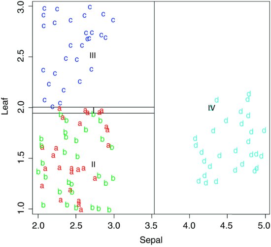
You see that taxa III and IV are beautifully separated on the basis of sepal length and leaf width, but taxa I and II are all jumbled up (recall that they are separated from one another on the basis of petiole length).
23.8 Testing for the existence of humps
Tree models can be useful in assessing whether or not there is a hump in the relationship between y and x. This is difficult to do using other kinds of regression, because linear models seldom distinguish between humps and asymptotes. If a tree model puts a lower section at the right of the graph than in the centre, then this hints at the presence of a hump in the data. Likewise, if it puts an elevated section at the left-hand end of the x axis then that is indicative of a U-shaped function.
Here is a function called hump which extracts information from a tree model to draw the stepped function through a scatterplot:
hump <- function(x,y){

library(tree)

model <- tree(y∼x)

xs <- grep("[0-9]",model[[1]][[5]])

xv <- as.numeric(substring(model[[1]][[5]][xs],2,10))

xv <- xv[1:(length(xv)/2)]

xv <- c(min(x),sort(xv),max(x))

yv <- model[[1]][[4]][model[[1]][[1]]=="<leaf>"]

plot(x,y,col="red",pch=16,
xlab=deparse(substitute(x)),ylab=deparse(substitute(y)))

i <- 1

j <- 2

k <- 1

b <- 2*length(yv)+1

for (a in 1:b){

lines(c(xv[i],xv[j]),c(yv[k],yv[i]))

if (a %% 2 == 0){

j <- j+1

k <- k+1}

else{

i <- i+1

}}}
We shall test it on the ethanol data which are definitely humped (p. 675):
library(lattice)

attach(ethanol)

names(ethanol)
[1] "NOx" "C" "E"
hump(E,NOx)

There is a minimum number of points necessary for creating a new step (n = 5), and a minimum difference in the mean of one group and the next. To see this, you should contrast these two fits:
hump(E[E<1.007],NOx[E<1.007])
hump(E[E<1.006],NOx[E<1.006])
The first data set has evidence of a hump, but the second does not.