Chapter 26

Spatial Statistics

There are three kinds of problems that you might tackle with spatial statistics:

• point processes (locations and spatial patterns of individuals);
• maps of a continuous response variable (kriging);
• spatially explicit responses affected by the identity, size and proximity of neighbours.

26.1 Point processes

There are three broad classes of spatial pattern on a continuum from complete regularity (evenly spaced hexagons where every individual is the same distance from its nearest neighbour) to complete aggregation (all the individuals clustered into a single clump): we call these regular, random and aggregated patterns and they look like this: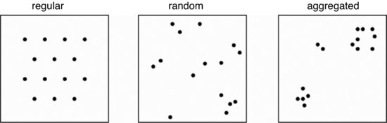

In their simplest form, the data consist of sets of x and y coordinates within some sampling frame such as a square or a circle in which the individuals have been mapped. The first question is often whether there is any evidence to allow rejection of the null hypothesis of complete spatial randomness (CSR). In a random pattern the distribution of each individual is completely independent of the distribution of every other. Individuals neither inhibit nor promote one another. In a regular pattern individuals are more spaced out than in a random one, presumably because of some mechanism (such as competition) that eliminates individuals that are too close together. In an aggregated pattern, individual are more clumped than in a random one, presumably because of some process such as reproduction with limited dispersal, or because of underlying spatial heterogeneity (e.g. good patches and bad patches).

Counts of individuals within sample areas (quadrats) can be analysed by comparing the frequency distribution of counts with a Poisson distribution with the same mean. Aggregated spatial patterns (in which the variance is greater than the mean) are often well described by a negative binomial distribution with aggregation parameter k (see p. 315). The main problem with quadrat-based counts is that they are highly scale-dependent. The same spatial pattern could appear to be regular when analysed with small quadrats, aggregated when analysed with medium-sized quadrats, yet random when analysed with large quadrats.

Distance measures are of two broad types: measures from individuals to their nearest neighbours, and measures from random points to the nearest individual. Recall that the nearest individual to a random point is not a randomly selected individual: this protocol favours selection of isolated individuals and individuals on the edges of clumps.

In other circumstances, you might be willing to take the existence of patchiness for granted, and to carry out a more sophisticated analysis of the spatial attributes of the patches themselves, their mean size and the variance in size, spatial variation in the spacing of patches of different sizes, and so on.

26.1.1 Random points in a circle

The circle is specified by the x and y coordinates of its centre and by the radius. We can compute the coordinates of the circumference of a circle of radius r, with its centre located at x = y = 0 like this

x <- r*sin(angle)

y <- r*cos(angle)

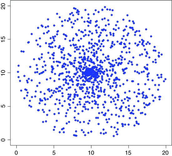
where angle varies between 0 and 2π radians. There are two ways to generate random points within this circle: one is to assume that the circle is a target, and that I am aiming at the centre; and the other is to assume that I am cutting a circular patch out of a sea of spatially independent points. In the first case we might generate a uniformly random angle, then generate a uniformly distributed random distance along this radius. Overall, these points will cluster around the centre of the circle because the random radii are most densely clustered here.

point <- function(r) {

angle <- runif(1)*2*pi

length <- runif(1)*r

x <- length*sin(angle)

y <- length*cos(angle)

return (data.frame(x,y))

}

The easting and northing of the centre of the circle are e0 and n0 respectively, the radius is r and we want to plot 1000 random points within the circle:

e0 <- 10

n0 <- 10

plot(e0,n0,ylab="",xlab="",ylim=c(0,2*n0),xlim=c(0,2*e0),type="n")

 

n <- 1000

r <- 10

 

for (i in 1:n) {

a <- point(r)

e <- e0+a[1]

n <- n0+a[2]

points(e,n,pch=16,col="blue")

}

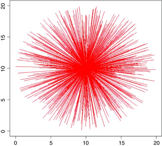
If, instead of plotting the random points, you draw lines from the centre of the circle to the random points, you can see exactly why this algorithm gives random points that are clustered around the centre.

e0 <- 10

n0 <- 10

plot(e0,n0,ylab="",xlab="",ylim=c(0,2*n0),xlim=c(0,2*e0),type="n")

 

n <- 1000

r <- 10

 

for (i in 1:n) {

a <- point(r)

e <- e0+a[1]

n <- n0+a[2]

lines(c(e0,e),c(n0,n),col= "red")

}

A different question is the ‘cookie cutter’ case. If I throw a circular quadrat onto a spatially uniform map of random points, what does the distribution of my randomly selected points look like? Here is the pseudo-code:

• Make a square map of n random points (uniform eastings and uniform northings).
• Make a polygon to describe the circumference of your circular sampling quadrat.
• Put the quadrat on the square map, and use the function from maptools to ask whether or not every point on the map is, or is not, inside your circle (the function is called point.in.polygon and returns a 1 for TRUE and a zero for FALSE).
• Use the output vector called wanted to select the points that are in your circle

Here is the R code for 10 000 random points in a square region whose side is of length 10:

n <- 10000

side <- 10

 

library(maptools)

 

space <- cbind((runif(n)*side),(runif(n)*side))

plot(space)

 

circle <- function(e,n,r) {

angle <- seq(0,2*pi,2*pi/360)

x - r*sin(angle)

y - r*cos(angle)

return (cbind((x+e),(y+n)))

}

Select the random points in a circle of radius 1 centred at (8, 8):

xc - 8

yc <- 8

rc <- 1

 

outline <- circle(xc,yc,rc)

 

wanted <- point.in.polygon(space[,1],space[,2],outline[,1],outline[,2])

 

points(space[,1][wanted==1],space[,2][wanted==1], col="blue",pch=16)

Now add a bigger red circle of points centred at (5, 5):

xc <- 5

yc <- 5

rc <- 2

 

outline<-circle(xc,yc,rc)

 

wanted<-point.in.polygon(space[,1],space[,2],outline[,1],outline[,2])

 

points(space[,1][wanted==1],space[,2][wanted==1], col="red",pch=16)

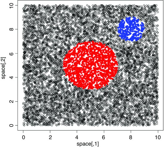
As intended, there is no clustering of these points around the centres of the circles. If the circle represents a small fraction of the total area of the square, then this method is very inefficient.

26.2 Nearest neighbours

Suppose that we have been set the problem of drawing lines to join the nearest neighbour pairs of any given set of points (x, y) that are mapped in two dimensions. There are three steps to the computing: we need to

• compute the distance to every neighbour;
• identify the smallest neighbour distance for each individual;
• use these minimal distances to identify all the nearest neighbours.

We start by generating a random spatial distribution of 100 individuals by simulating their x and y coordinates from a uniform probability distribution:

x <- runif(100)

y <- runif(100)

The graphics parameter pty="s" makes the plotting area square, as we would want for a map like this:

par(pty="s")

plot(x,y,pch=21,bg="red")

Computing the distances is straightforward: for each individual we use Pythagoras to calculate the distance to every other plant. The distance between two points with coordinates (x1, y1) and (x2, y2) is d:

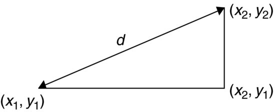
The square on the hypotenuse (d2) is the sum of the squares on the two adjacent sides: (x2−x1)2+(y2−y1)2 so the distance d is given by

We write a function for this as follows:

distance <- function(x1,y1,x2,y2) sqrt((x2 - x1)^2 + (y2 - y1)^2)

Now we loop through each individual i and calculate a vector of distances, d, from every other individual. The nearest neighbour distance is the minimum value of d, and the identity of the nearest neighbour, nn, is found using the which function, which(d==min(d[-i])), which gives the subscript of the minimum value of d (the [-i] is necessary to exclude the distance 0 which results from the ith individual's distance from itself). Here is the complete code to compute nearest neighbour distances, r, and identities, nn, for all 100 individuals on the map:

r <- numeric(100)

nn <- numeric(100)

d <- numeric(100)

for (i in 1:100) {

for (k in 1:100) d[k] <- distance(x[i],y[i],x[k],y[k])

r[i] <- min(d[-i])

nn[i] <- which(d==min(d[-i]))

}

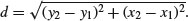
Now we can fulfil the brief, and draw lines to join each individual to its nearest neighbour, like this:

for (i in 1:100) lines(c(x[i],x[nn[i]]),c(y[i],y[nn[i]]),col="green")

Note that when two points are very close together, and each is the nearest neighbour of the other, it can look as if a single point is not joined to any neighbours.

The next task is to work out how many of the individuals are closer to the edge of the area than they are to their nearest neighbour. Because the bottom and left margins are at y = 0 and x = 0 respectively, the y coordinate of any point gives the distance from the bottom edge of the area and the x coordinate gives the distance from the left-hand margin. We need only work out the distance of each individual from the top and right-hand margins of the area:

topd <- 1-y

rightd <- 1-x

Now we use the parallel minimum function pmin to work out the distance to the nearest margin for each of the 100 individuals:

edge <- pmin(x,y,topd,rightd)

Finally, we count the number of cases where the distance to the edge is less than the distance to the nearest neighbour:

sum(edge<r)

[1] 25 

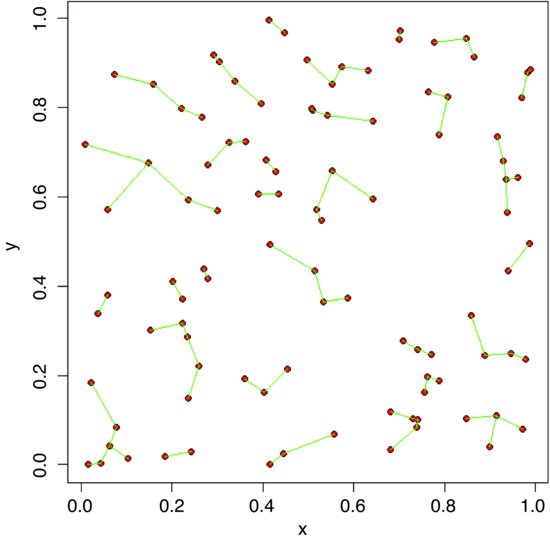
We identify these points on the map by circling them in red:

plot(x,y,pch=16)

id <- which(edge<r)

points(x[id],y[id],col="red",cex=1.5,lwd=2)

It is the vertical or horizontal distance to the edge that has been used to identify these points, so some of them look suspiciously close to their neighbours (e.g. in the bottom left-hand corner).

Edge effects are potentially very important in spatial point processes, especially when there are few individuals or the mapped area is long and thin (rather than square or circular). Excluding the individuals that are closer to the edge than to their nearest neighbour reduces the mean nearest neighbour distance:

mean(r)

[1] 0.05294168

mean(r[-id])

[1] 0.04802602

26.2.1 Tessellation

The procedure of splitting a two-dimensional surface into a mosaic by halving the distance between neighbouring pairs of points is called tessellation. There is a function to do this in the tripack package by Albrecht Gebhardt:

install.packages("tripack")

library(tripack)

x<-runif(100)

y<-runif(100)

Create a Voronoi object (here called map) by applying the function called voronoi.mosaic to the vectors of x and y coordinates.

map<-voronoi.mosaic(x,y)

Start by producing a scatterplot of the random points (in green):

plot(x,y,pch=16,col="green")

Now add the Voronoi tesselation on top of the scatterplot:

plot.voronoi(map,pch=16,add=TRUE)

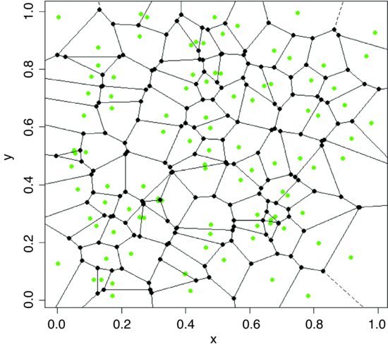
As you can see, it is relatively unusual for the points to be in the ‘centre of gravity’ of their tessellated patch. Each node (black circle) is a circumcircle centre of some triangle from the Delaunay triangulation.

26.3 Tests for spatial randomness

Clark and Evans (1954) give a very simple test of spatial randomness. Making the strong assumption that you know the population density of the individuals, (generally you do not know this, and would need to estimate it independently), then the expected mean distance to the nearest neighbour is

In our example we have 100 individuals in a unit square, so and E(r) = 0.05. The actual mean nearest neighbour distance was

mean(r)

[1] 0.05294168

which is very close to expectation: this clearly is a random distribution of individuals (as we constructed it to be). An index of randomness is given by the ratio 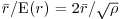. This takes the value 1 for random patterns, more than 1 for regular (spaced-out) patterns, and less than 1 for aggregated patterns.

One problem with such first-order estimates of spatial pattern (including measures such as the variance–mean ratio) is that they can give no feel for the way that spatial distribution changes within an area.

26.3.1 Ripley's K

The second-order properties of a spatial point process describe the way that spatial interactions change through space. These are computationally intensive measures that take a range of distances within the area, calculate a pattern measure, then plot a graph of the function against distance, to show how the pattern measure changes with scale. The most widely used second-order measure is the K function, which is defined as

where is the mean number of points per unit area (the intensity of the pattern). If there is no spatial dependence, then the expected number of points that are within a distance d of an arbitrary point is times the mean density. So, if the mean density is 2 points per square metre , then the expected number of points within a 5 m radius is . If there is clustering, then we expect an excess of points at short distances (i.e. for small d). Likewise, for a regularly spaced pattern, we expect an excess of long distances, and hence few individuals at short distances (i.e. ). Ripley's K (published in 1976) is calculated as follows:

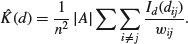
Here n is the number of points in region A with area |A|, and dij are the distances between points (the distance between the ith and jth points, to be precise). To account for edge effects, the model includes the term wij which is the fraction of the area, centred on i and passing through j, that lies within the area A (all the wij are 1 for points that lie well away from the edges of the area). Id(dij) is an indicator function to show which points are to be counted as neighbours at this value of d: it takes the value 1 if and zero otherwise (i.e. points with dij>d are omitted from the summation). The pattern measure is obtained by plotting against d . This is then compared with the curve that would be observed under complete spatial randomness (namely, a plot of against d). When clustering occurs, and the curve lies above the CSR curve, while regular patterns produce a curve below the CSR curve.

You can see why you need the edge correction from this simple simulation experiment. For individual number 1, with coordinates (x1, y1), calculate the distances to all the other individuals, using the function distance that we wrote earlier (p. 830):

distances <- numeric(100)

for(i in 1:100) distances[i] <- distance(x[1],y[1],x[i],y[i])

Now find out how many other individuals are within a distance d of this individual. Take as an example d = 0.1.

sum(distances<0.1)-1

[1] 4

There were four other individuals within a distance d = 0.1 of the first individual (the distance 0 from itself is included in the sum, so we have to correct for this by subtracting 1). The next step is to generalize the procedure from this one individual to all the individuals. We make a two-dimensional matrix called dd to contain all the distances from every individual (rows) to every other individual (columns):

dd <- numeric(10000)

dd <- matrix(dd,nrow=100)

The matrix of distances is computed within loops for both individual (j) and neighbour (i) like this:

for (j in 1:100) {for(i in 1:100) dd[j,i] <- distance(x[j],y[j],x[i],y[i])}

Alternatively, you could use sapply with an anonymous function like this, which has the advantage that we do not need to prepare the matrix dd in advance:

dd <- sapply(1:100,function (i,j=1:100) distance(x[j],y[j],x[i],y[i]))

We should check that the number of individuals within 0.1 of individual 1 is still 4 under this new notation. Note the use of blank subscripts [1,] to mean ‘all the individuals in row number 1’:

sum(dd[1,]<0.1)-1

[1] 4

So that's OK. We want to calculate the sum of this quantity over all individuals, not just individual number 1:

sum(dd<0.1)-100

[1] 270

This means that there are 270 cases in which other individuals are counted within d = 0.1 of focal individuals. Next, create a vector containing a range of different distances, d, over which we want to calculate K(d) by counting the number of individuals within distance d, summed over all individuals:

d <- seq(0.01,1,0.01)

For each of these distances we need to work out the total number of neighbours of all individuals. So, in place of 0.1 (in the sum, above), we need to put each of the d values in turn. The count of individuals is going to be a vector of length 100 (one for each d):

count <- numeric(100)

Calculate the count for each distance d:

for (i in 1:100) count[i] <- sum(dd<d[i])-100

The expected count increases with d as so we scale our count by dividing by the square of the total number of individuals n2 = 1002 = 10 000:

K <- count/10000

Finally, plot a graph of K against d:

plot(d,K,type="l",col="red")

Not surprisingly, when we sample the whole area (d = 1), we count all of the individuals in every neighbourhood (K = 1). For CSR the graph should follow so we add a line to show this:

lines(d,pi*d^2,col="blue")

Up to about d = 0.2 the agreement between the two lines is reasonably good, but for longer distances our algorithm is counting far too few neighbours. This is because much of the area scanned around marginal individuals is invisible, since it lies outside the study area (there may well be individuals out there, but we shall never know). This simple model demonstrates that the edge correction is a fundamental part of Ripley's K.

Fortunately, we do not have to write a function to work out a corrected value for K; it is available as Kfn in the built-in spatial library. Here we use it to analyse the pattern of trees in the dataframe called pines. The library function ppinit reads the data from a library file called pines.dat which is stored in the spatial/ppdata directory. It then converts this into a list with names $x, $y and $area. The first row of the file contains the number of trees (71) the second row has the name of the data set (pines), the third row has the four boundaries of the region plus the scaling factor (0, 96, 0, 100, 10 so that the coordinates of lower and upper x are computed as 0 and 9.6, and the coordinates of lower and upper y are 0 and 10). The remaining rows of the data file contain x and y coordinates for each individual tree, and these are converted into a list of x values and a separate list of y values. You need to know these details about the structure of the data files in order to use these library functions with your own data (see p. 845).

library(spatial)

pines <- ppinit("pines.dat")

First, set up the plotting area with two square frames:

windows(7,4)

par(mfrow=c(1,2),pty="s")

On the left, make a map using the x and y locations of the trees, and on the right make a plot of L(t) (the pattern measure) against distance:

plot(pines,pch=16, col="blue")

plot(Kfn(pines,5),type="s",xlab="distance",ylab="L(t)")

Recall that if there was CSR, then the expected value of K would be ; to linearize this, we could divide by and then take the square root. This is the measure used in the function Kfn, where it is called 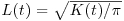. Now for the simulated upper and lower bounds: the first argument in Kenvl (calculating envelopes for K) is the maximum distance (half the length of one side), the second is the number of simulations (100 is usually sufficient), and the third is the number of individuals within the mapped area (71 pine trees in this case).

lims <- Kenvl(5,100,Psim(71))

lines(lims$x,lims$lower,lty=2,col="red")

lines(lims$x,lims$upper,lty=2,col="red")

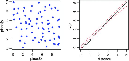
There is a suggestion that at relatively small distances (around 1 or so), the trees are rather regularly distributed (more spaced out than random), because the plot of L(t) against distance falls below the lower envelope of the CSR line (it should lie between the two limits for its whole length if there was CSR). The mechanism underlying this spatial regularity (e.g. non-random recruitment or mortality, competition between growing trees, or underlying non-randomness in the substrate) would need to be investigated in detail. With an aggregated pattern, the line would fall above the upper envelope (see p. 847).

26.3.2 Quadrat-based methods

Another approach to testing for spatial randomness is to count the number of individuals in quadrats of different sizes. Here, the quadrats have an area of 0.01, so the expected number per quadrat is 1. Earlier, we generated 100 random coordinates for x and y:

plot(x,y,pch=16,col="red")

grid(10,10,lty=1)

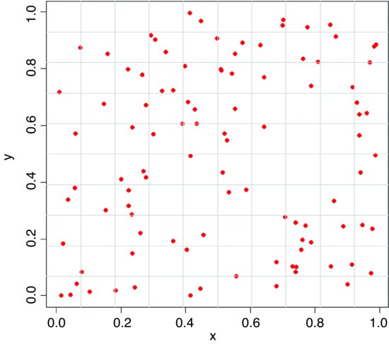
Note that the grid function has not done exactly what we intended (the grids are not exactly on the tick marks). To count the numbers of individuals in each of the cells of the map, the trick is to use cut to convert the x and y coordinates of the map into bin numbers (between 1 and 10 for the quadrat size we have drawn here). To achieve this, the break points are generated by the sequence (0,1,0.1):

xt <- cut(x,seq(0,1,0.1))

yt <- cut(y,seq(0,1,0.1))

This creates vectors of integer subscripts between 1 and 10 for xt and yt. Now all we need to do is use table to count up the number of individuals in every cell (i.e. in every combination of xt and yt):

count <- as.vector (table(xt,yt))

table(count)

count

 0	1	2	3	4	5

37	38	16	7	1	1 

This shows that 37 cells are empty, 1 cell had five individuals, but no cells contained six or more individuals. Now we need to see what this distribution would look like under a particular null hypothesis. For a Poisson process (see p. 314), for example,

Note that the mean depends upon the quadrat size we have chosen. With 100 individuals in the whole area, the expected number in any one of our 100 cells, , is 1.0. The expected frequencies of counts between 0 and 5 are therefore given by

(expected <- 100*exp(-1)/sapply(0:5,factorial))

 [1] 36.7879441 36.7879441 18.3939721 6.1313240 1.5328310 0.3065662 

The fit between observed and expected is almost perfect (as we should expect, of course, having generated the random pattern ourselves). A test of the significance of the difference between an observed and expected frequency distribution is shown on p. 841.

26.3.3 Aggregated pattern and quadrat count data

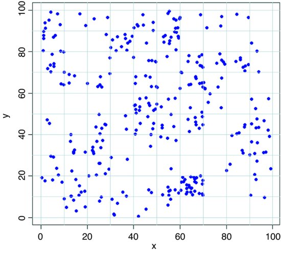
Here is an example of a quadrat-based analysis of an aggregated spatial pattern. We begin by producing a map of the trees, then use abline rather than grid (see above) to make sure that the lines are exactly where we want them to be:

trees <- read.table("c:\\temp\\trees.txt",header=T)

attach(trees)

names(trees)

[1] "x" "y"

plot(x,y,pch=16,col="blue")

abline(v=seq(0,100,10),col="lightgray",lty=1)

abline(h=seq(0,100,10),col="lightgray",lty=1)

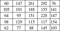
We cut up the data and tabulate the counts:

xt <- cut(x,10)

yt <- cut(y,10)

count <- as.vector(table(xt,yt))

table(count)

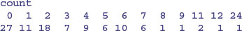
There are quadrats with as many as 24 individuals, and despite the fact that the mean number is greater than 3 individuals per square, there are still 27 completely empty squares. The expected frequencies under the null hypothesis of a random pattern depend only on the mean number per cell,

mean(count)

[1] 3.11

and as a preliminary estimate of the departure from randomness we calculate the variance–mean ratio (recall that with the Poisson distribution the variance is equal to the mean):

var(count)/mean(count)

[1] 4.007243

These data are distinctly aggregated (the variance–mean ratio is much greater than 1), so we might compare the counts with a negative binomial distribution (p. 315). The expected frequencies are estimated by multiplying our total number of squares (100) by the probability densities from a negative binomial distribution generated by the function dnbinom. This has three arguments: the counts for which we want the probabilities (0:10), the mean (mu=3.11) and the aggregation parameter k = mu^2/(var-mu) = size=1.03417:

mean(count)^2/(var(count)- mean(count))

[1] 1.03417

Here are the expected frequencies:

(expected <- dnbinom(0:10, size=1.03417, mu=3.11)*100)

[1] 23.798804 18.470128 14.097756 10.700189 8.098573 6.119123

[7] 4.618259 3.482699 2.624761 1.977235 1.488890

These are reasonably close to the observed frequencies (above) but we need to quantify the lack of fit. The plan is to display the observed and expected frequencies as pairs of bars, side by side. We need to make space, therefore, to accommodate, say, 22 bars (11 for each histogram):

ht <- numeric(22)

observed <- table(count)

ht[seq(1,21,2)] <- observed

ht[seq(2,22,2)] <- expected

names <- rep("",22)

names[seq(1,21,2)] <- as.character(0:10)

barplot(ht,col=c("darkgray","lightgray"),names=names,

 	ylab="frequency",xlab="trees per quadrat")

legend(locator(1),legend=c("observed","expected"),

 	fill=c("darkgray","lightgray"))

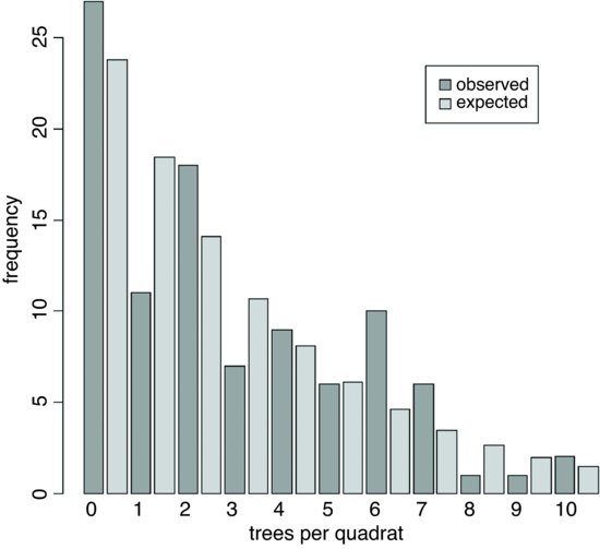
The fit is reasonably good, but we need a quantitative estimate of the lack of agreement between the observed and expected distributions. Pearson's chi-squared is perhaps the simplest (p. 367). We need to trim the observed and expected vectors so that none of the expected frequencies is less than 4. Inspection shows that the lowest expected frequency greater than 4 is in location 7, so we shall accumulate all frequencies in locations 8 and above

expected[8] <- sum(expected[8:length(expected)])

expected <- expected[-c(9:length(expected))]

observed[8] <- sum(observed[8:length(observed)])

observed <- observed[-c(9:length(observed))]

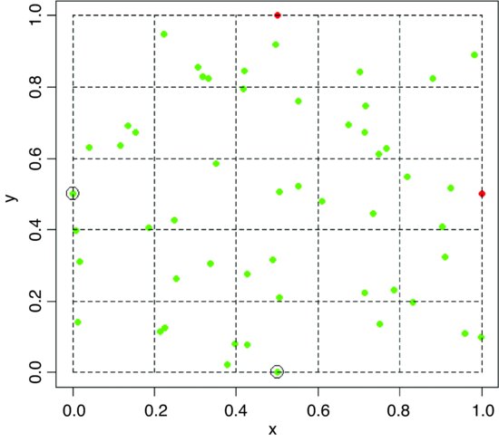
Now calculate Pearson's chi-squared as :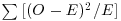

sum((observed-expected)^2/expected)

[1] 12.80059

The number of degrees of freedom is the number of legitimate comparisons (8) minus the number of parameters estimated from the data (2) minus 1 for contingency (i.e. 8 – 2 – 1 = 5 d.f.). So the probability of obtaining a chi-squared value of this size (12.8) or greater is

1-pchisq(12.8,5)

[1] 0.02532684

We conclude that the negative binomial is an imperfect description of these quadrat data (because p < 0.05). The reason for the significant lack of fit is the serious underestimation of quadrats containing just one tree, and the excess of quadrats containing six or seven trees.

26.3.4 Counting things on maps

The convention is that if a point falls exactly on the x axis or exactly on the y axis, then it is counted as being inside the area (green points on the map below), but if it falls on the top axis or on the right hand axis, then it is outside the area (red points).

plot(c(0,2),c(0,2),type="n",xlab="",ylab="")

lines(c(0,1,1,0,0),c(0,0,1,1,0))

points(c(0.5,0),c(0,0.5),pch=16,col="green",cex=1.5)

points(c(0.5,1),c(1,0.5),pch=16,col="red",cex=1.5)

That way, all points on the map have an equal probability of being counted, and there is no double-counting of points. Red points on the top axis will be counted in the next quadrat to the north, and red points on the right hand axis will be counted in the next quadrat to the east.

This counting convention is embodied in the R function called cut, using round brackets and square brackets like this: "(b1, b2]", "(b2, b3]" … for the default right = TRUE; here, the round bracket means ‘greater than’ and the square bracket means ‘less than or equal to’. For our convention, we need to specify right=FALSE. Now we have "[b1, b2)", "[b2, b3)" … where the square bracket means ‘greater than or equal to’ and the round bracket means ‘less than’. Here are some test data:

data <- read.table("c:\\temp\\countpoints.txt",header=T)

attach(data)

plot(x,y,pch=16,col="green")

points(x[y==1 | x==1],y[y==1 | x==1],pch=16,col="red")

lines(c(0,1,1,0,0),c(0,0,1,1,0),lty=2)

lines(c(0.2,0.2),c(0,1),lty=2)

lines(c(0.4,0.4),c(0,1),lty=2)

lines(c(0.6,0.6),c(0,1),lty=2)

lines(c(0.8,0.8),c(0,1),lty=2)

lines(c(0,1),c(0.2,0.2),lty=2)

lines(c(0,1),c(0.4,0.4),lty=2)

lines(c(0,1),c(0.6,0.6),lty=2)

lines(c(0,1),c(0.8,0.8),lty=2)

points(0,0.5,cex=2)

points(0.5,0,cex=2)

We want to count the number of points in each of 25 quadrats measuring 0.2 × 0.2. The function to achieve this is cut. We need to specify six values at which to cut the x axis and six values at which to cut the y axis. The function converts the vector of continuous values of x into a factor xc with five levels (and converts the coordinates y into factor levels within yc in the same way):

xc <- cut(x,seq(0,1,0.2),right = FALSE)

yc <- cut(y,seq(0,1,0.2),right = FALSE)

We count the number of points in each quadrat using table, like this:

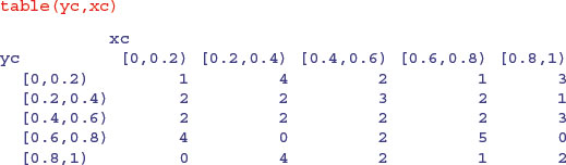
which gives the correct counts, but in a pattern that does not match the map (the y values are upside down). We can fix this by reordering the factor levels of yc using rev to reverse the order of the rows:

yc <- factor(yc,rev(levels(yc)))

Now, table produces a map-like summary of the counts:

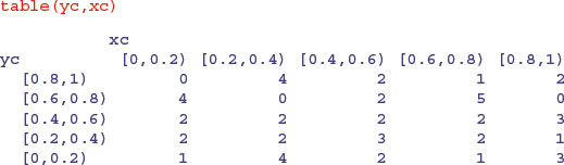
There are four points on the edge of the map: the red points are not counted (totals 2 and 3 respectively), but the circled green points are counted (totals 2 and 2, above).

26.4 Packages for spatial statistics

In addition to the built-in library spatial there are two substantial contributed packages for analysing spatial data. The spatstat library is what you need for the statistical analysis of spatial point patterns, while the spdep library is good for the spatial analysis of data from mapped regions.

With point patterns the things you will want to do include

• creation, manipulation and plotting of point patterns,
• exploratory data analysis,
• simulation of point process models,
• parametric model fitting,
• hypothesis tests and diagnostics;

whereas with maps you might

• compute basic spatial statistics such as Moran's I and Geary's C,
• create neighbour objects of class nb,
• create weights list objects of class lw,
• work out neighbour relations from polygons (outlines of regions),
• colour mapped regions on the basis of derived statistics.

You need to take time to master the different formats of the data objects used by the two packages. You will waste a lot of time if you try to use the functions in these libraries with your own, unreconstructed data files.

Here is the code for installing and reading about spatstat and spdep:

install.packages("spatstat")

library(help=spatstat)

library(spatstat)

demo(spatstat)

 	

install.packages("spdep")

library(help=spdep)

library(spdep)

26.4.1 The spatstat package

You need to use the function ppp to convert your coordinate data into an object of class ppp representing a point pattern data set in the two-dimensional plane. Our next dataframe contains information on the locations and sizes of 3359 ragwort plants in a 30 m × 15 m map:

data <- read.table("c:\\temp\\ragwortmap.txt",header=T)

attach(data)

names(data)

[1] "xcoord" "ycoord" "type" 

The plants are classified as belonging to one of four types: skeletons are dead stems of plants that flowered the year before, regrowth are skeletons that have live shoots at the base, seedlings are small plants (a few weeks old) and rosettes are larger plants (one or more years old) destined to flower this year. The function ppp requires separate vectors for the x and y coordinates: these are in our file under the names xcoord and ycoord. The third and fourth arguments to ppp are the boundary coordinates for x and y respectively (in this example c(0,3000) for x and c(0,1500) for y). The final argument to ppp contains a vector of what are known as ‘marks’: these are the factor levels associated with each of the points (in this case, type is either skeleton, regrowth, seedling or rosette). You give a name to the ppp object (ragwort) and define it like this:

ragwort <- ppp(xcoord,ycoord,c(0,3000),c(0,1500),marks=type)

You can now use the object called ragwort in a host of different functions for plotting and statistical modelling within the spatstat library. For instance, here are maps of the point patterns for the four plant types separately:

plot(split(ragwort),main="")

Point patterns are summarized like this:

summary(ragwort)

Marked planar point pattern: 3359 points

Average intensity 0.000746 points per square unit

Multitype:

		frequency		proportion	intensity

regrowth		135		0.0402		3.00e-05

rosette		146		0.0435		3.24e-05

seedling		1100		0.3270		2.44e-04

skeleton		1980		0.5890		4.40e-04

 	

Window: rectangle = [0, 3000]x[0, 1500]units

Window area = 4500000 square units 

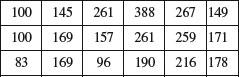
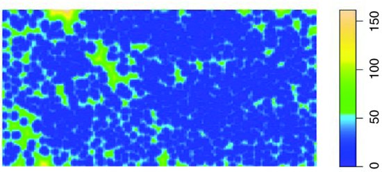
which computes the frequency and intensity for each mark (‘intensity’ is the mean density of points per unit area). In this case, where distances are in centimetres, the intensity is the mean number of plants per square centimetre (the highest intensity is skeletons, with 0.000 44 cm–2). The function quadratcount produces a useful summary of counts:

plot(quadratcount(ragwort),main="")

This is the default, but you can specify either the numbers of quadrats in the x and y directions (default 5 and 5), or provide numeric vectors giving the x and y coordinates of the boundaries of the quadrats. If we want counts in 0.5 m squares:

plot(quadratcount(ragwort,

 	xbreaks=c(0,500,1000,1500,2000,2500,3000),

 	ybreaks=c(0,500,1000,1500)),main="")

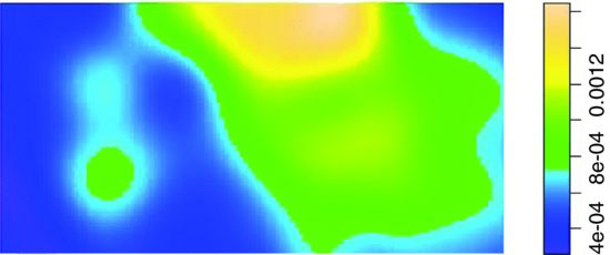
There are functions for producing density plots of the point pattern:

Z <- density.ppp(ragwort)

plot(Z,main="")

The classic graphical description of spatial point patterns is Ripley's K (see p. 834).

K <- Kest(ragwort)

plot(K, main = "K function")

The red dotted line shows the expected number of plants within a radius r of a plant under the assumption of complete spatial randomness. The observed curve (black) lies above this line, indicating strong spatial aggregation at all spatial scales up to more than 300 cm.

The pair correlation function pcf for the ragwort data looks like this:

pc <- pcf(ragwort)

plot(pc, main = "Pair correlation function")

There is strong correlation between pairs of plants at small scales, but much less above r = 20 cm. The function distmap shows the distance map around individual plants:

Z <- distmap(ragwort)

plot(Z,main="")

You can use spatstat to generate a wide range of patterns of random points, including independent uniform random points, inhomogeneous Poisson point processes, inhibition processes, and Gibbs point processes using Metropolis–Hastings (see ?spatstat for details). Some useful functions on point-to-point distances in spatstat include:

nndist	nearest neighbour distances;
nnwhich	find nearest neighbours;
pairdist	distances between all pairs of points;
crossdist	distances between points in two patterns;
exactdt	distance from any location to nearest data point;
distmap	distance map image;
density.ppp	kernel smoothed density.

There are several summary statistics for a multi-type point pattern with a component $marks which is a factor:

Gcross, Gdot, Gmulti	multitype nearest neighbour distributions;
Kcross, Kdot, Kmulti	multitype K-functions;
Jcross, Jdot, Jmulti	multitype J-functions;
Alltypes	estimates of the above for all i,j pairs;
Lest	multitype I-function;
Kcross.inhom	inhomogeneous counterpart of Kcross;
Kdot.inhom	inhomogeneous counterpart of Kdot.

Point process models are fitted using the ppm function like this:

model <- ppm(ragwort, ∼marks + polynom(x, y, 2), Poisson())

plot(model)

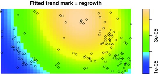
There are eight such maps produced, showing means (four maps) and standard errors (four maps). Typing

summary(model)

produces a massive table of output, including what the authors refer to as the ‘gory details’.

26.4.2 The spdep package

The key to using this package is to understand the differences between the various formats in which the spatial data can be held:

• x and y coordinates (in a two-column matrix, with x in column 1 and y in 2);
• lists of regions that are neighbours to each region, with (potentially) unequal numbers of neighbours in different cases (this is called a neighbour file and belongs to class nb);
• dataframes containing a region, its neighbour and the statistical weight of the association between the two regions on each row (class data.frame);
• lists containing the identities of the k nearest neighbours (class knn);
• a weights list object suitable for computing Moran's I or Geary's C (class lw);
• lists of polygons, defining the outlines of regions on a map (class polylist).

Unlike spatstat (Section 26.4.1) where the x and y coordinates were in separate vectors, spdep wants the x and y coordinates in a single two-column matrix. For the ragwort data (p. 845) we need to write:

library(spdep)

myco <- cbind(xcoord,ycoord)

myco <- matrix(myco,ncol=2)

A raw list of coordinates contains no information about neighbours, but we can use the knearneigh function to convert a matrix of coordinates into an object of class knn. Here we ask for the four nearest neighbours of each plant:

myco.knn <- knearneigh(myco, k=4)

This list object has the following structure:

str(myco.knn)

List of 5

 $ nn		: int [1:3359, 1:4] 2 1 4 3 7 4 8 7 10 9 …

 $ np		: int 3359

 $ k			: num 4

 $ dimension	: int 2

 $ x			: num [1:3359, 1:2] 27 29 20 20 78 25 89 97 253 259 …

 - attr(*, "class")= chr "knn"

 - attr(*, "call")= language knearneigh(x = myco, k = 4)

• $nn contains 3359 lists, each a vector of length 4, containing the identities of the four points that are the nearest neighbours of each of the points from 1 to 3359.
• $np (an integer) is the number of points in the pattern.
• $k is the number of neighbours of each point.
• $dimension is 2.
• $x is the matrix of coordinates of each point (x in the first column, y in the second).

Before you can do much with a knn object you will typically want to convert it to a neighbour object (nb) using the knn2nb function like this:

myco.nb <- knn2nb(myco.knn)

The essential concept for using the spdep package is the neighbour object (with class nb). For a given location, typically identified by the (x, y) coordinates of its centroid, the neighbour object is a list, with the elements of the list numbered from 1 to the number of locations, and each element of the list contains a vector of integers representing the identities of the locations that share a boundary with that location. The important point is that different vectors are likely to be of different lengths. You can do interesting things with nb objects. Here is a plot with each point joined to its four nearest neighbours – you specify the nb object and the matrix of coordinates:

plot(myco.nb,myco)

The simplest way to create an nb object is to read a text file containing one row for each neighbour relationship, using the special input function read.gwt2nb. The header row can take one of two forms. The simplest (called ‘old-style GWT’) is a single integer giving the number of locations in the file. There will always be many more rows in the data file than this number, because each location will typically have several neighbours. The second form of the header row has four elements: the first is set arbitrarily to zero, the second is the integer number of locations, the third is the name of the shape object and the fourth is the vector of names identifying the locations. An example should make this clear. These are the contents of a text file called naydf.txt:

5

1	2 	1

1 	3 	1

2 	1 	1

2 	3 	1

2 	4 	1

3 	1 	1

3 	2 	1

3 	5 	1

4 	2 	1

4 	3 	1

4 	5 	1

5 	3 	1

5 	4 	1

The 5 in the first row indicates that this file contains information on five locations. On subsequent lines the first number identifies the location, the second number identifies one of its neighbours, and the third number is the weight of that relationship. Thus, location 5 has just two neighbours, and they are locations 3 and 4 (the last two rows of the file). We create a neighbour object for these data with the read.gwt2nb function like this:

dd <- read.gwt2nb("c:\\temp\\naydf.txt")

Here is a summary of the newly-created neighbour object called dd:

summary(dd)

Neighbour list object:

Number of regions: 5

Number of nonzero links: 13

Percentage nonzero weights: 52

Average number of links: 2.6

Non-symmetric neighbours list

Link number distribution:

 	

2 3

2 3

2 least connected regions:

1 5 with 2 links

3 most connected regions:

2 3 4 with 3 links

Here are the five vectors of neighbours:

dd[[1]]

[1] 2 3

dd[[2]]

[1] 1 3 4

dd[[3]]

[1] 1 2 5

dd[[4]]

[1] 2 3 5

dd[[5]]

[1] 3 4

The coordinates of the five locations need to be specified:

coox <- c(1,2,3,4,5)

cooy <- c(3,1,2,0,3)

and the vectors of coordinates need to be combined into a two-column matrix. Now we can use plot with dd and the coordinate matrix to indicate the neighbour relations of all five locations like this:

plot(dd,matrix(cbind(coox,cooy),ncol=2))

text(coox,cooy,as.character(1:5),pos=rep(3,5))

Note the use of pos = 3 to position the location numbers 1 to 5 above their points. You can see that locations 1 and 5 are the least connected (two neighbours) and location 3 is the most connected (four neighbours). Note that the specification in the data file was not fully reciprocal, because location 4 was defined as a neighbour of location 3 but not vice versa. There is a comment, Non-symmetric neighbours list, in the output to summary(dd) to draw attention to this. A function make.sym.nb(dd) is available to convert the object dd into a symmetric neighbours list.

For calculating indices much as Moran's I and Geary's C you need a ‘weights list’ object. This is created most simply from a neighbour object using the function nb2listw. For the ragwort data, we have already created a neighbour object called myco.nb (p. 850) and we create the weights list object myco.lw like this:

myco.lw <- nb2listw(myco.nb, style="W")

myco.lw

Characteristics of weights list object:

Neighbour list object:

Number of regions: 3359

Number of nonzero links: 13436

Percentage nonzero weights: 0.1190831

Average number of links: 4

Non-symmetric neighbours list

 	

Weights style: W

Weights constants summary:

 	n		nn	S0		S1	S2

W 3359	11282881 3359 1458.25 14077.88

There are three classic tests based on spatial cross products C(i, j), where z(i) = (x(i) –mean (x))/sd(x):

• Moran (C(i, j) = z(i)z(j));
• Geary (C(i, j) = (z(i)−z(j))2);
• Sokal (C(i, j) = |z(i)−z(j)|).

Here is the Moran I test for the ragwort data, using the weights list object myco.lw:

moran(1:3359,myco.lw,length(myco.nb),Szero(myco.lw))

$I

[1] 0.9931224

 	

$K

[1] 1.8

Here is Geary's C for the same data:

geary(1:3359,myco.lw,length(myco.nb),length(myco.nb)-1,Szero(myco.lw))

$C

[1] 0.004549794

 	

$K

[1] 1.8

Here is Mantel's permutation test:

sp.mantel.mc(1:3359,myco.lw,nsim=99)

	Mantel permutation test for moran measure

data: 1:3359

weights: myco.lw

number of simulations + 1: 100

 	

statistic = 3334.905, observed rank = 100, p-value = 0.01

alternative hypothesis: greater

sample estimates:

mean of permutations	sd of permutations

 	-5.434839			34.012539 

In all cases, the first argument is a vector of location numbers (1 to 3359 in the ragwort example), the second argument is the weight list object myco.lw. For moran, the third argument is the length of the neighbours object, length(myco.nb) and the fourth is Szero(myco.lw), the global sum of weights, both of which evaluate to 3359 in this case. The function geary has an extra argument, length(myco.nb)-1, and sp.mantel.mc specifies the number of simulations.

26.4.3 Polygon lists

Perhaps the most complex spatial data handled by spdep comprise digitized outlines (sets of x and y coordinates) defining multiple regions, each of which can be interpreted by R as a polygon. Here is such a list from the built-in columbus data set:

data(columbus)

polys

The polys object is of class polylist and comprises a list of 49 polygons. Here is the first of them:

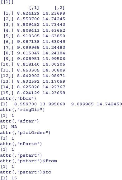
Each element of the list contains a two-column matrix with x coordinates in column 1 and y coordinates in column 2, with as many rows as there are digitized points on the outline of the polygon in question. After the matrix of coordinates come the boundary box and various plotting options.

There is an extremely useful function poly2nb that takes the list of polygons and works out which regions are neighbours of one another by looking for shared boundaries. The result is an nb object (here called colnbs), and we can get a visual check of how well poly2nb has worked by overlaying the neighbour relations on a map of the polygon outlines:

colnbs <- poly2nb(polys)

plot(c(5.5,11.5),c(10.5,15),type="n",xlab="",ylab="")

for (i in 1:49) polygon(polys[[i]][,1],polys[[i]][,2],col="lightgrey")

plot(colnbs,coords,add=T,col="red")

The agreement is perfect. Obviously, creating a polygon list is likely to be a huge amount of work, especially if there are many regions, each with complicated outlines. Before you start making one, you should check that it has not been done already by someone else who might be willing to share it with you. To create polygon lists and bounding boxes from imported shape files you should use one of read.shapefile or Map2poly (for details, see ?read.shapefile and ?Map2poly). Subtleties include the facts that lakes are digitized anti-clockwise and islands are digitized clockwise.

26.5 Geostatistical data

Mapped data commonly show the value of a continuous response variable (e.g. the concentration of a mineral ore) at different spatial locations. The fundamental problem with this kind of data is spatial pseudoreplication. Hot spots tend to generate lots of data, and these data tend to be rather similar because they come from essentially the same place. Cold spots are poorly represented and typically widely separated. Large areas between the cold spots have no data at all.

Spatial statistics takes account of this spatial autocorrelation in various ways. The fundament tool of spatial statistics is the variogram (or semivariogram). This measures how quickly spatial autocorrelation, , falls off with increasing distance:

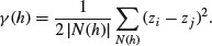
Here N(h) is the set of all pairwise Euclidean distances i – j = h, | N(h) | is the number of distinct pairs within N(h), and zi and zj are values of the response variable at spatial locations i and j. There are two important rules of thumb: (1) the distance of reliability of the variogram is less than half the maximum distance over the entire field of data; and (2) you should only consider producing an empirical variogram when you have more than 30 data points on the map.

Plots of the empirical variogram against distance are characterized by some quaintly named features which give away its origin in geological prospecting:

• nugget, small-scale variation plus measurement error;
• sill, the asymptotic value of as , representing the variance of the random field;
• range, the threshold distance (if such exists) beyond which the data are no longer autocorrelated.

Variogram plots that do not asymptote may be symptomatic of trended data or a non-stationary stochastic process. The covariogram C(h) is the covariance of z values at separation h, for all i and i + h within the maximum distance over the whole field of data:

The correlogram is a ratio of covariances:

Here C(0) is the variance of the random field and is the variogram. Where the variogram increases with distance, the correlogram and covariogram decline with distance.

The variogram assumes that the data are untrended. If there are trends, then one option is median polishing. This involves modelling row and column effects from the map like this:

y ∼ overall mean + row effect + column effect + residual

This two-way model assumes additive effects and would not work if there was an interaction between the rows and columns of the map. An alternative would be to use a generalized additive model (p. 670) with non-parametric smoothers for latitude and longitude.

Anisotropy occurs when spatial autocorrelation changes with direction. If the sill changes with direction, this is called zonal anisotropy. When it is the range that changes with direction, the process is called geometric anisotropy.

Geographers have a wonderful knack of making the simplest ideas sound complicated. Kriging is nothing more than linear interpolation through space. Ordinary kriging uses a random function model of spatial correlation to calculate a weighted linear combination of the available samples to predict the response for an unmeasured location. Universal kriging is a modification of ordinary kriging that allows for spatial trends. We say no more about models for spatial prediction here; details can be found in Kaluzny et al. (1998). Our concern is with using spatial information in the interpretation of experimental or observational studies that have a single response variable. The emphasis is on using location-specific measurements to model the spatial autocorrelation structure of the data.

The idea of a variogram is to illustrate the way in which spatial variance increases with spatial scale (or alternatively, how correlation between neighbours falls off with distance). Confusingly, R has two functions with the same name: variogram (lower-case ‘v’) is in the spatial library and Variogram (upper-case ‘V’) is in nlme. Their usage is contrasted here for the ragwort data (p. 845).

To use variogram from the spatial library, you need to create a trend surface or a kriging object with columns x, y and z. The first two columns are the spatial coordinates, while the third contains the response variable (basal stem diameter in the case of the ragwort data):

library(spatial)

data <- read.table("c:\\temp\\ragwortmap2006.txt",header=T)

attach(data)

names(data)

[1] "stems" "diameter" "xcoord" "ycoord"

dts <- data.frame(x=xcoord,y=ycoord,z=diameter)

Next, you need to create a trend surface using a function such as surf.ls:

surface <- surf.ls(2,dts)

This trend surface object is then the first argument to variogram, followed by the number of bins (here 300). The function computes the average squared difference for pairs with separation in each bin, returning results for bins that contain six or more pairs:

variogram(surface,300)

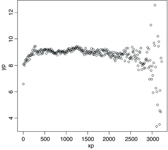
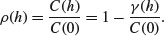
The sister function is correlogram, which takes identical arguments:

correlogram(surface,300)

The positive correlations have disappeared by about 100 cm. The correlations at xp = 3000 are spurious edge effects.

For the Variogram function in the nlme library, you need to fit a model (typically using gls or lme), then provide the model object along with a form function in the call:

library(nlme)

model <- gls(diameter∼xcoord+ycoord)

plot(Variogram(model,form= ∼xcoord+ycoord))

26.6 Regression models with spatially correlated errors: Generalized least squares

In Chapter 19 we looked at the use of linear mixed-effects models for dealing with random effects and temporal pseudoreplication. Here we illustrate the use of generalized least squares (GLS) for regression modelling where we would expect neighbouring values of the response variable to be correlated. The great advantage of the gls function is that the errors are allowed to be correlated and/or to have unequal variances. The gls function is part of the nlme package:

library(nlme)

The following example is a geographic-scale trial to compare the yields of 56 different varieties of wheat. What makes the analysis more challenging is that the farms carrying out the trial were spread out over a wide range of latitudes and longitudes.

spatialdata <- read.table("c:\\temp\\spatialdata.txt",header=T)

attach(spatialdata)

names(spatialdata)

[1] "Block" "variety" "yield" "latitude" "longitude"

We begin with graphical data inspection to see the effect of location on yield:

windows(7,4)

par(mfrow=c(1,2))

plot(latitude,yield,pch=21,col="blue",bg="red")

plot(longitude,yield,pch=21,col="blue",bg="red")

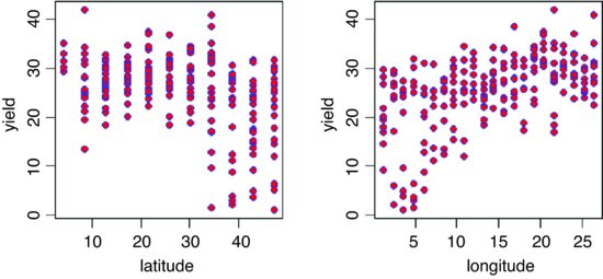
There are clearly big effects of latitude and longitude on both the mean yield and the variance in yield. The latitude effect looks like a threshold effect, with little impact for latitudes less than 30. The longitude effect looks more continuous but there is a hint of non-linearity (perhaps even a hump). The varieties differ substantially in their mean yields:

windows(7,7)

barplot(sort(tapply(yield,variety,mean)),col="green")

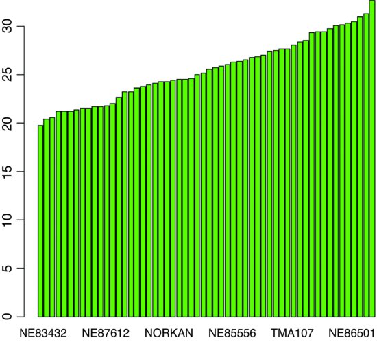
The lowest-yielding varieties are producing about 20 and the highest about 30 kg of grain per unit area. There are also substantial block effects on yield:

tapply(yield,Block,mean)

	1		2		3		4	 

27.57500	28.81091 24.42589 21.42807 

Here is the simplest possible analysis – a one-way analysis of variance using variety as the only explanatory variable:

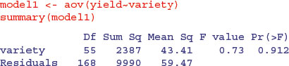
This says that there are no significant differences between the yields of the 56 varieties. We can try a split-plot analysis (see p. 519) using varieties nested within blocks:

Block <- factor(Block)

model2 <- aov(yield∼Block+variety+Error(Block))

summary(model2)

Error: Block

 	Df Sum Sq Mean Sq

Block 3	1854	617.9

 	

Error: Within

		Df	Sum Sq Mean Sq F	value	Pr(>F)

variety	55	2389		43.43	0.881	0.702

Residuals	165	8135		49.30 

This has made no difference to our interpretation. We could fit latitude and longitude as covariates:

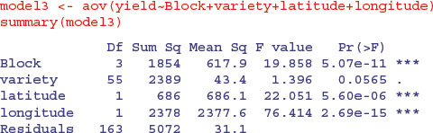
This makes an enormous difference. Now the differences between varieties are close to significance (p = 0.0565).

Finally, we could use a GLS model to introduce spatial covariance between yields from locations that are close together. We begin by making a grouped data object:

space <- groupedData(yield∼variety|Block)

We use this to fit a model using gls which allows the errors to be correlated and to have unequal variances. We shall add these sophistications later:

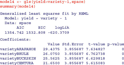
and so on, for all 56 varieties. The variety means are given, rather than differences between means, because we removed the intercept from the model by using yield∼variety-1 rather than yield∼variety in the model formula (see p. 398).

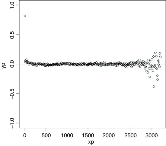
Now we want to include the spatial covariance. The Variogram function is applied to model4 like this:

plot(Variogram(model4,form=∼latitude+longitude))

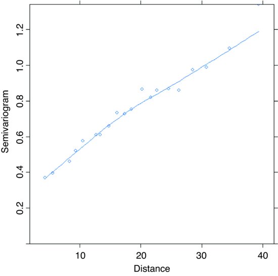
Table 26.1 Spatial correlation structures. Options for specifying the form and distance dependence of spatial correlation in generalized least squares models. For more detail, see the help on ?corClasses and on the individual correlation structures (e.g. ?corExp).

corExp	exponential spatial correlation
corGaus	Gaussian spatial correlation
corLin	linear spatial correlation
corRatio	rational quadratic spatial correlation
corSpher	spherical spatial correlation
corSymm	general correlation matrix, with no additional structure

The sample variogram increases with distance, illustrating the expected spatial correlation. Extrapolating back to zero distance, there appears to be a nugget of about 0.2. There are several assumptions we could make about the spatial correlation in these data. For instance, we could try a spherical correlation structure, using the corSpher class (the range of options for spatial correlation structure is shown in Table 26.1). We need to specify the distance at which the semivariogram first reaches 1. Inspection shows this distance to be about 28. We can update model4 to include this information:

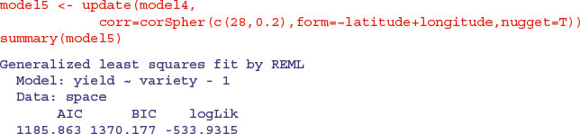
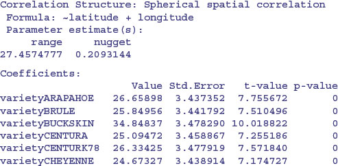
This is a big improvement, and AIC has dropped from 1354.742 to 1185.863. The range (27.46) and nugget (0.209) are very close to our visual estimates.

There are other kinds of spatial model, of course. We might try a rational quadratic model (corRatio); this needs an estimate of the distance at which the semivariogram is (1 + nugget)/2 = 1.2/2 = 0.6, as well as an estimate of the nugget. Inspection gives a distance of about 12.5, so we write:

model6 <- update(model4,

corr=corRatio(c(12.5,0.2),form=∼latitude+longitude,nugget=T))

We can use anova to compare the two spatial models:

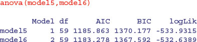
The rational quadratic model (model6) has the lower AIC and is therefore preferred to the spherical model. To test for the significance of the spatial correlation parameters we need to compare the preferred spatial model6 with the non-spatial model4 (which assumed spatially independent errors):

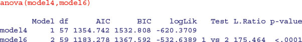
The two extra degrees of freedom used up in accounting for the spatial structure are clearly justified. We need to check the adequacy of the corRatio model. This is done by inspection of the sample variogram for the normalized residuals of model6:

plot(Variogram(model6,resType="n"))

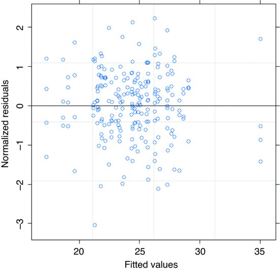
There is no pattern in the plot of the sample variogram, so we conclude that the rational quadratic is adequate. To check for constancy of variance, we can plot the normalized residuals against the fitted values like this:

plot(model6,resid( ., type="n")∼fitted(.),abline=0)

and the normal plot is obtained in the usual way:

qqnorm(model6,∼resid(.,type="n"))

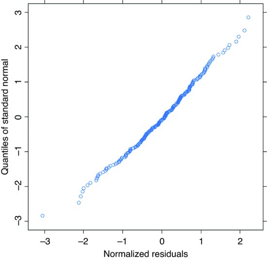
The model looks fine.

The next step is to investigate the significance of any differences between the varieties. Use update to change the structure of the model from yield∼variety-1 to yield∼variety:

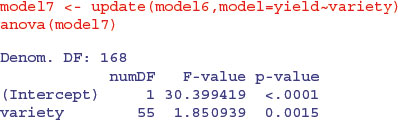
The differences between the varieties now appear to be highly significant (recall that they were only marginally significant with our linear model3 using analysis of covariance to take account of the latitude and longitude effects). Specific contrasts between varieties can be carried out using the L argument to anova. Suppose that we want to compare the mean yields of the first and third varieties. To do this, we set up a vector of contrast coefficients c(-1,0,1) and apply the contrast like this:

anova(model6,L=c(-1,0,1))

Denom. DF: 168 

 	F-test for linear combination(s)

varietyARAPAHOE varietyBUCKSKIN 

 	-1			1 

 	numDF F-value p-value

1		1 7.696728 0.0062

Note that we use model6 (with all the variety means), not model7 (with an intercept and Helmert contrasts). The specified varieties, Arapahoe and Buckskin, exhibit highly significant differences in mean yield.

26.7 Creating a dot-distribution map from a relational database

Here is an example of extracting a relatively small subset of data from a large relational database, and using the information to produce a dot distribution map. The Access database contains two related tables:

• sites contains information on 2628 locations;
• records contains lists of species found at each site (43 001 in total).

The two tables are related by a variable called site number. The task is to extract eastings and northings for each record of a named species, and use these to produce a dot-distribution map, with one dot for each site at which that particular species was recorded.

Instructions on how to make an open database connection are on p. 154. I assume that you have downloaded the Access database called berks.accdb from this book's website (see p. iii) and created an ODBC channel called berks on your computer. Open the channel to connect R to the Access database, using the function odbcConnect:

library(RODBC)

channel <- odbcConnect("berks") 

To complete the map you need to:

• read a file of x and y coordinates for the outline of the region being mapped (the county of Berkshire in this example);
• draw the outline on a plot without any labelling on the axes;
• use axis to label using single digits (the grid references have 5 digits);
• add a grid using abline with grey lines;
• specify a species to map;
• read the coordinates for this species into R from the Access database;
• use points to add the distribution dots to the map.

Here is the outline of the county of Berkshire:

data<-read.table("c:\\temp\\vc22outline.txt",header=T)

attach(data)

Now plot the outline of the county on blank axes:

plot(e,n,type="l",xaxt="n",yaxt="n",xlab="",ylab="")

The next task is to label the 100 km squares with a single digit on each of the axes:

axis(1,seq(20000,100000,10000),seq(2,10,1))

axis(2,seq(60000,110000,10000),seq(6,11,1))

Produce a grid for the 100 km squares in grey:

abline(v=10000*(2:10),col="gray")

abline(h=10000*(6:11),col="gray")

Use the mouse to stretch or contract the left and bottom margins of the graphics window until the grids make perfect squares.

Next, write a function called mapit to specify the name of the species whose data you want to extract from the database, and use this name to construct a query that will extract information for all of the sites at which the named species is found. Finally, execute the query using sqlQuery to create a dataframe in R containing the necessary eastings and northings (the x and y coordinates for the dots to be added to the map):

mapit <- function(x) {

mapname <- x

query <- paste(

"SELECT sites.easting, sites.northing

 FROM records

 INNER JOIN sites ON records.site=sites.[site number]

 WHERE records.trimmed ='", mapname, "'", sep='')

mysites <- sqlQuery(channel, query)

with(mysites,points(easting,northing,pch=16,col="red"))

}

The two tables in the database are related by shared variables called site and site number, respectively. The square brackets deal with the gap in the variable name. Run the function by specifying the name of the species you want to map (Viscum album):

mapit("Viscum album")

This will extract the coordinates and add the distribution dots to the map in red:

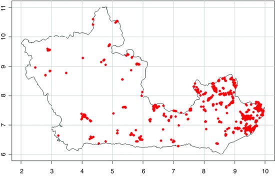
Note how the variable name (mapname, which is "Viscum album" in this example) has been incorporated into the WHERE part of the query using the paste function. The way the two tables, sites and records, are related is specified in the INNER JOIN part of the query. The longer of the two tables (records) is specified in the FROM part of the query. The key here is in dealing correctly with the single quotes that need to appear around the species name inside the WHERE part of the query character string.