Chapter 28
Simulation Models
Simulation modelling is an enormous topic, and all I intend here is to demonstrate a few very simple temporal and spatial simulation techniques that give the flavour of what is possible in R.
Simulation models are used for investigating dynamics in time, in space, or in both space and time together. For temporal dynamics we might be interested in:
- the transient dynamics (the behaviour after the start but before equilibrium is attained – if indeed equilibrium is ever attained);
- equilibrium behaviour (after the transients have damped away);
- chaos (random-looking, but actually deterministic temporal dynamics that are extremely sensitive to initial conditions).
For spatial dynamics, we might use simulation models to study:
- metapopulation dynamics (where local extinction and recolonization of patches characterize the long-term behaviour, with constant turnover of occupied patches);
- neighbour relations (in spatially explicit systems where the performance of individuals is determined by the identity and attributes of their immediate neighbours);
- pattern generation (dynamical processes that lead to the generation of emergent, but more or less coherent patterns).
28.1 Temporal dynamics: Chaotic dynamics in population size
Biological populations typically increase exponentially when they are small, but individuals perform less well as population density rises, because of competition, predation or disease. In aggregate, these effects on birth and death rates are called density-dependent processes, and it is the nature of the density-dependent processes that determines the temporal pattern of population dynamics. The simplest density-dependent model of population dynamics is known as the quadratic map. It is a first-order non-linear difference equation,

where N(t) is the population size at time t, N(t+1) is the population size at time t+1, and the single parameter, λ, is known as the per-capita multiplication rate. The population can only increase when the population is small if λ > 1, the so-called invasion criterion. But how does the system behave as λ increases above 1?
We begin by simulating time series of populations for different values of λ and plotting them to see what happens. First, here are the dynamics with λ = 2:
par(mfrow=c(2,2))
lambda <- 2
x <- numeric(40)
x[1] <- 0.6
for (t in 2 : 40) x[t] <- lambda * x[t-1] * (1 - x[t-1])
plot(1:40,x,type="l",ylim=c(0,1),ylab="population",
xlab="time",main="lambda = 2.0")
The population falls very quickly from its initial value (0.6) to equilibrium (N* = 0.5) and stays there; this system has a stable point equilibrium. What if λ were to increase to 3.3?
lambda <- 3.3
x <- numeric(40)
x[1] <- 0.6
for (t in 2 : 40) x[t] <- lambda * x[t-1] * (1 - x[t-1])
plot(1:40,x,type="l",ylim=c(0,1),ylab="population",
xlab="time",main="lambda = 3.3")
Now the dynamics show persistent two-point cycles. What about λ = 3.5?
lambda <- 3.5
x <- numeric(40)
x[1] <- 0.6
for (t in 2 : 40) x[t] <- lambda * x[t-1] * (1 - x[t-1])
plot(1:40,x,type="l",ylim=c(0,1),ylab="population",
xlab="time",main="lambda = 3.5")
The outcome is qualitatively different. Now we have persistent four-point cycles. Suppose that λ were to increase to 4:
lambda <- 4
x <- numeric(40)
x[1] <- 0.6
for (t in 2 : 40) x[t] <- lambda * x[t-1] * (1 - x[t-1])
plot(1:40,x,type="l",ylim=c(0,1),ylab="population",
xlab="time",main="lambda = 4.0")
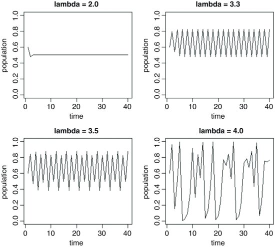
Now this is really interesting. The dynamics do not repeat in any easily described pattern. They are said to be chaotic because the pattern shows extreme sensitivity to initial conditions: tiny changes in initial conditions can have huge consequences on numbers at a given time in the future.
28.1.1 Investigating the route to chaos
We have seen four snapshots of the relationship between λ and population dynamics. To investigate this more fully, we should write a function to describe the dynamics as a function of λ, and extract a set of (say, 20) sequential population densities, after any transients have died away (after, say, 380 iterations):
numbers <- function (lambda) {
x <- numeric(400)
x[1] <- 0.6
for (t in 2 : 400) x[t] <- lambda * x[t-1] * (1 - x[t-1])
x[381:400] }
The idea is to plot these 20 values on the y axis of a new graph, against the value of λ that produced them. A stable point equilibrium will be represented by a single point, because all 20 values of y will be identical. Two-point cycles will show up as two points, four-point cycles as four points, but chaotic systems will appear as many points. Start with a blank graph:
par(mfrow=c(1,1))
plot(c(2,4),c(0,1),type="n",xlab="lambda",ylab="population")
Now, simulate using a for loop a wide range of values for λ between 2 and 4 (the range we investigated earlier), use the function sapply to apply our function to the current value of λ, and then use points to add these results to the graph:
for(lam in seq(2,4,0.01))
points(rep(lam,20),sapply(lam,numbers),pch=16,cex=0.5,col="blue")
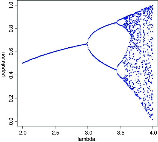
This graph shows what is called ‘the period-doubling route to chaos’; see May (1976) for details.
28.2 Temporal and spatial dynamics: A simulated random walk in two dimensions
The idea is to follow an individual as it staggers its way around a two-dimensional random walk, starting at the point (50, 50) and leaving a trail of lines on a square surface which scales from 0 to 100. First, we need to define what we mean by our random walk. Suppose that in the x direction the individual could move one step to the left in a given time period, stay exactly where it is for the whole time period, or move one step to the right. We need to specify the probabilities of these three outcomes. Likewise, in the y direction the individual could move one step up in a given time period, stay exactly where it is for the whole time period, or move one step down. Again, we need to specify probabilities. In R, the three movement options are c(1,0,-1) for each of the types of motion (left, stay or right, and up, stay or down) and we might as well say that each of the three motions is equally likely. We need to select one of the three motions at random independently for the x and y directions at each time period. In R we use the sample function for this:
sample(c(1,0,-1),1)
which selects one value (the last argument is 1) with equal probability from the three listed options (+1, 0 or –1). Out of 99 repeats of this procedure, we should expect an average of 33 ups and 33 downs, 33 lefts and 33 rights.
We begin by defining the axes and drawing the start position in red:
plot(0:100,0:100,type="n",xlab="",ylab="")
x <- y <- 50
points(50,50,pch=16,col="red",cex=1.5)
Now simulate the spatial dynamics of the random walk with up to 10 000 time steps:
for (i in 1:10000) {
xi <- sample(c(1,0,-1),1)
yi <- sample(c(1,0,-1),1)
lines(c(x,x+xi),c(y,y+yi),col="blue")
x <- x+xi
y <- y+yi
if (x>100 | x<0 | y>100 | y<0) break
}
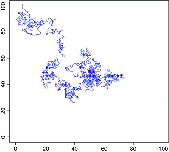
You could make the walk more sophisticated by providing wrap-around margins (see below). On average, of course, the random walk should stay in the middle, where it started, but as you will see by running this model repeatedly, most random walks do nothing of the sort. Instead, they wander off and fall over one of the edges in more or less short order.
28.3 Spatial simulation models
There are two broad types of spatial simulation models:
- spatial models that are divided but not spatially explicit;
- spatially explicit models where neighbours can be important.
Metapopulation dynamics is a classic example of a spatial model that is not spatially explicit. Patches are occupied or not, but the fate of a patch is not related to the fate of its immediate neighbours but rather by the global supply of propagules generated by all the occupied patches in the entire metapopulation.
28.3.1 Metapopulation dynamics
The theory is very simple. The world is divided up into many patches, all of which are potentially habitable. Populations on inhabited patches go extinct with a density-independent probability, e. Occupied patches all contain the same population density, and produce migrants (propagules) at a rate m per patch. Empty patches are colonized at a rate proportional to the total density of propagules and the availability of empty patches that are suitable for colonization. The response variable is the proportion of patches that are occupied, p. The dynamics of p, therefore, are just gains minus losses, so
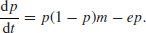
At equilibrium dp/dt = 0, and so
giving the equilibrium proportion of occupied patches p* as

This draws attention to a critical result: there is a threshold migration rate (m = e) below which the metapopulation cannot persist, and the proportion of occupied patches will drift inexorably to zero. Above this threshold, the metapopulation persists in dynamic equilibrium with patches continually going extinct (the mean lifetime of a patch is 1/e) and other patches becoming colonized by immigrant propagules. This model is due to Levins (1969).
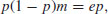
The simulation produces a moving cartoon of the occupied (yellow) and empty patches (red). We begin by setting the parameter values
m <- 0.15
e <- 0.1
We create a square universe of 10 000 patches in a 100×100 array, but this is not a spatially explicit model, and so the map-like aspects of the image should be ignored. The response variable is just the proportion of all patches that are occupied. Here are the initial conditions, placing occupied 100 patches at random in a sea of unoccupied patches:
s <- (1-e)
N <- matrix(rep(0,10000),nrow=100)
xs <- sample(1:100)
ys <- sample(1:100)
for (i in 1:100){
N[xs[i],ys[i]] <- 1 }
image(1:100,1:100,N)
We want the simulation to run over 1000 generations:
for (t in 1:1000){
First we model the survival (or not) of occupied patches. Each cell of the universe gets an independent random number from a uniform distribution (a real number between 0 and 1). If the random number is bigger than or equal to the survival rate s (= 1 – e, above) then the patch survives for another generation. If the random number is less than s, then the patch goes extinct and N is set to zero:
S <- matrix(runif(10000),nrow=100)
N <- N*(S<s)
Note that this one statement updates the whole matrix of 10 000 patches. Next, we work out the production of propagules, im, by the surviving patches (the rate per patch is m):
im <- floor(sum( N*m))
We assume that the settlement of the propagules is random, some falling in empty patches but others being ‘wasted’ by falling in already occupied patches:
placed <- matrix(sample(c(rep(1,im) ,rep (0,10000-im))),nrow=100)
N <- N+placed
N <- apply(N,2,function(x) ifelse(x>1,1,x))
The last line is necessary to keep the values of N just 0 (empty) or 1 (occupied) because our algorithm gives N = 2 when a propagule falls in an occupied patch. Now we can draw the map of the occupied patches:
image(1:100,1:100,N,add=TRUE)
box(col="red")
}
Because the migration rate (m = 0.15) exceeds the extinction rate (e = 0.1) the metapopulation is predicted to persist. The analytical solution for the long-term proportion of patches occupied is one-third of patches (1 – 0.1/0.15 = 0.333). At any particular time of stopping the simulation, you can work out the actual proportion occupancy as
sum(N)/length(N)
[1] 0.268
because there were 2680 occupied patches in this map at the time we stopped. Here is the code in one block:
m <- 0.15
e <- 0.1
s <- (1-e)
N <- matrix(rep(0,10000),nrow=100)
xs <- sample(1:100)
ys <- sample(1:100)
for (i in 1:100){
N[xs[i],ys[i]] <- 1 }
image(1:100,1:100,N)
for (t in 1:1000){
S <- matrix(runif(10000),nrow=100)
N <- N*(S<s)
im <- floor(sum( N*m))
placed <- matrix(sample(c(rep(1,im) ,rep (0,10000-im))),nrow=100)
N <- N+placed
N <- apply(N,2,function(x) ifelse(x>1,1,x))
image(1:100,1:100,N,add=TRUE)
box(col="red")
}
Remember that a metapopulation model is not spatially explicit, so you should not read anything into any the apparent neighbour relations in this graph (the occupied patches should be distributed at random over the surface).
28.3.2 Coexistence resulting from spatially explicit (local) density dependence
We have two species which would not coexist in a well-mixed environment because the fecundity of species A is greater than the fecundity of species B, and this would lead, sooner or later, to the competitive exclusion of species B and the persistence of a monoculture of species A. The idea is to see whether the introduction of local neighbourhood density dependence is sufficient to prevent competitive exclusion and allow long-term coexistence of the two species.
The kind of mechanism that might allow such an outcome is the build-up of specialist natural enemies such as insect herbivores or fungal pathogens in the vicinity of groups of adults of species A, that might prevent recruitment by species A when there were more than a threshold number, say T, of individuals of species A in a neighbourhood.
The problem with spatially explicit models is that we have to model what happens at the edges of the universe. All locations need to have the same numbers of neighbours in the model, but patches on the edge have fewer neighbours than those in the middle. The simplest solution is to model the universe as having ‘wrap-around margins’ in which the left-hand edge is assumed to have the right-hand edge as its left-hand neighbour (and vice versa), while the top edge is assumed to have the bottom edge as its neighbour above (and vice versa). The four corners of the universe are assumed to be reciprocal diagonal neighbours.
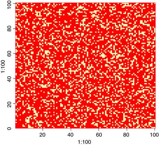
We need to define who is a neighbour of whom. The simplest method, adopted here, is to assume a square grid in which a central cell has eight neighbours – three above, three below and one to either side:
plot(c(0,1),c(0,1),xaxt="n",yaxt="n",type="n",xlab="",ylab="")
abline("v"=c(1/3,2/3))
abline("h"=c(1/3,2/3))
xs <- c(.15,.5,.85,.15,.85,.15,.5,.85)
ys <- c(.85,.85,.85,.5,.5,.15,.15,.15)
for (i in 1:8) text(xs[i],ys[i],as.character(i))
text(.5,.5,"target cell")
This code produces a plot showing a target cell in the centre of a matrix, and the numbers in the other cells indicate its ‘first-order neighbours’:
We need to write a function to define the margins for cells on the top, bottom and edge of our universe, N, and which determines all the neighbours of the four corner cells. Our universe is 100×100 cells and so the matrix containing all the neighbours will need to be 102×102. Note the use of subscripts (see p. 36 for revision of this):
margins <- function(N){
edges <- matrix(rep(0,10404),nrow=102)
edges[2:101,2:101] <- N
edges[1,2:101] <- N[100,]
edges[102,2:101] <- N[1,]
edges[2:101,1] <- N[,100]
edges[2:101,102] <- N[,1]
edges[1,1] <- N[100,100]
edges[102,102] <- N[1,1]
edges[1,102] <- N[100,1]
edges[102,1] <- N[1,100]
edges}
Next, we need to write a function to count the number of species A in the eight neighbouring cells, for any cell i, j:
nhood <- function(X,j,i) sum(X[(j-1):(j+1),(i-1):(i+1)]==1)
Now we can set the parameter values: the reproductive rates of species A and B, the death rate of adults (which determines the space freed up for recruitment) and the threshold number, T, of species A (out of the eight neighbours) above which recruitment cannot occur:
Ra <- 3
Rb <- 2.0
D <- 0.25
s <- (1-D)
T <- 6
The initial conditions fill one half of the universe with species A and the other half with species B, so that we can watch any spatial pattern as it emerges:
N <- matrix(c(rep(1,5000),rep(2,5000)),nrow=100)
image(1:100,1:100,N)
We run the simulation for 1000 time steps:
for (t in 1:1000) {
First, we need to see if the occupant of a cell survives or dies. For this, we compare a uniformly distributed random number between 0 and 1 with the specified survival rate s = 1 - D. If the random number is less than s the occupant survives, if it is greater than s it dies:
S <- 1*(matrix(runif(10000),nrow=100)<s)
We kill the necessary number of cells to open up space for recruitment:
N <- N*S
space <- 10000-sum(S)
Next, we need to compute the neighbourhood density of A for every cell (using the wrap-around margins):
nt <- margins(N)
tots <- matrix(rep(0,10000),nrow=100)
for (a in 2:101) {
for (b in 2:101) {
tots[a-1,b-1] <- nhood(nt,a,b)
}}
The survivors produce seeds as follows:
seedsA <- sum(N==1)*Ra
seedsB <- sum(N==2)*Rb
all.seeds <- seedsA+seedsB
fA <- seedsA/all.seeds
fB <- 1-fA
Seeds settle over the universe at random:
setA <- ceiling(10000*fA)
placed <- matrix(sample(c(rep(1,setA) ,rep (2,10000-setA))),nrow=100)
Seeds only produce recruits in empty cells N[i,j]==0. If the winner of an empty cell (placed) is species B, then species B gets that cell: if(placed[i,j]= = 2) N[i,j] <- 2. If species A is supposed to win a cell, then we need to check that it has fewer than T neighbours of species A. If so, species A gets the cell. If not, the cell is forfeited to species B: if (tots[i,j]>=T) N[i,j] <- 2.
for (i in 1:100){
for(j in 1:100){
if (N[i,j] == 0 )
if(placed[i,j]== 2) N[i,j] <- 2
else
if (tots[i,j]>=T) N[i,j] <- 2
else N[i,j] <- 1
}}
Finally, we can draw the map, showing species A in red and species B in white:
image(1:100,1:100,N,add=TRUE)
box(col="red")}
You can watch as the initial half-and-half pattern breaks down, and species A increases in frequency at the expense of species B. Eventually, however, species A gets to the point where most of the cells have six or more neighbouring cells containing species A, and its recruitment begins to fail. At equilibrium, species B persists in isolated cells or in small (white) patches, where the cells have six or more occupants that belong to species A. The full code for the model is in the file called janzen.txt on the book's web site.
If you set the threshold T = 9, you can watch as species A drives species B to extinction. If you want to turn the tables, and see species B take over the universe, set T = 0.
28.4 Pattern generation resulting from dynamic interactions
In this section we look at an example of an ecological interaction between a species and its parasite. The interaction is unstable in a non-spatial model, with increasing oscillations in numbers leading quickly to extinction of the host species and then, in the next generation, its parasite. The non-spatial dynamics look like this:
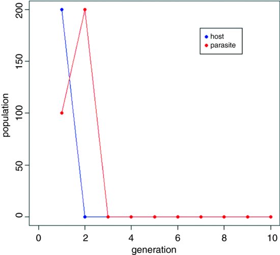
The parasite increases in generation number 1 and drives the host to extinction in generation 2, subsequently going extinct itself in generation 3. The challenge is to see if making the interaction spatially explicit can promote coexistence, and if so, through what pattern of spatial and temporal dynamics.
In a spatial model, we allow that hosts and parasites can move from the location in which they were born to any one of the eight first-order neighbouring cells (p. 901). For the purposes of dispersal, the universe is assumed to have wrap-around margins for both species. The interaction is interesting because it is capable of producing beautiful spatial patterns that fluctuate with host and parasite abundance. We begin by setting the parameter values for the dynamics of the host (r) and the parasite (a) and the migration rates of the host (Hmr=0.1) and parasite (Pmr=0.9). In this case the hosts are relatively sedentary and the parasites are highly mobile:
r <- 0.4
a <- 0.1
Hmr <- 0.1
Pmr <- 0.9
Next, we set up the matrices of host (N) and parasite (P) abundance. These will form what is termed a coupled map lattice:
N <- matrix(rep(0,10000),nrow=100)
P <- matrix(rep(0,10000),nrow=100)
The simulation is seeded by introducing 200 hosts and 100 parasites into a single cell at location [33,33]:
N[33,33] <- 200
P[33,33] <- 100
image(1:100,1:100,N)
We need to define a function called host to calculate the next host population as a function of current numbers of hosts and parasites (N and P), and another function called parasite to calculate the next parasite population as a function of N and P – this is called a Nicholson–Bailey model:
host <- function(N,P) N*exp(r-a*P)
parasite <- function(N,P) N*(1-exp(-a*P))
Both species need a definition of their wrap-around margins for defining the destinations of migrants from each cell:
host.edges <- function(N){
Hedges <- matrix(rep(0,10404),nrow=102)
Hedges[2:101,2:101] <- N
Hedges[1,2:101] <- N[100,]
Hedges[102,2:101] <- N[1,]
Hedges[2:101,1] <- N[,100]
Hedges[2:101,102] <- N[,1]
Hedges[1,1] <- N[100,100]
Hedges[102,102] <- N[1,1]
Hedges[1,102] <- N[100,1]
Hedges[102,1] <- N[1,100]
Hedges}
parasite.edges <- function(P){
Pedges <- matrix(rep(0,10404),nrow=102)
Pedges[2:101,2:101] <- P
Pedges[1,2:101] <- P[100,]
Pedges[102,2:101] <- P[1,]
Pedges[2:101,1] <- P[,100]
Pedges[2:101,102] <- P[,1]
Pedges[1,1] <- P[100,100]
Pedges[102,102] <- P[1,1]
Pedges[1,102] <- P[100,1]
Pedges[102,1] <- P[1,100]
Pedges}
A function is needed to define the eight cells that comprise the neighbourhood of any cell and add up the total number of neighbouring individuals:
nhood <- function(X,j,i) sum(X[(j-1):(j+1),(i-1):(i+1)])
The number of host migrants arriving in every cell is calculated as follows:
h.migration <- function(Hedges){
Hmigs <- matrix(rep(0,10000),nrow=100)
for (a in 2:101) {
for (b in 2:101) {
Hmigs[a-1,b-1] <- nhood(Hedges,a,b)
}}
Hmigs}
The number of parasite migrants is given by:
p.migration <- function(Pedges){
Pmigs <- matrix(rep(0,10000),nrow=100)
for (a in 2:101) {
for (b in 2:101) {
Pmigs[a-1,b-1] <- nhood(Pedges,a,b)
}}
Pmigs}
The simulation begins here, and runs for 600 generations:
for (t in 1:600){
he <- host.edges(N)
pe <- parasite.edges(P)
Hmigs <- h.migration(he)
Pmigs <- p.migration(pe)
N <- N-Hmr*N+Hmr*Hmigs/9
P <- P-Pmr*P+Pmr*Pmigs/9
Ni <- host(N,P)
P <- parasite(N,P)
N <- Ni
image(1:100,1:100,N,add=TRUE)
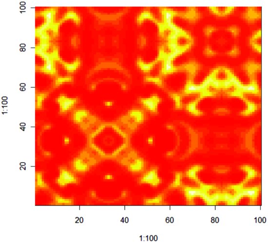
}
The full text of the R code is in a file called comins.txt on the book's web site. You can watch as the initial introduction at (33, 33) spreads out and both host and parasite populations pulse in abundance. Eventually, the wave of migration reaches the margin and appears on the right-hand edge. The fun starts when the two waves meet one another. The pattern below is typical of the structure that emerges towards the middle of a simulation run: