This time, will be using the Felzenszwalb algorithm, which is an unsupervised and efficient graph-based approach. It was proposed by P.F Felzenszwalb and Huttenlocher in 2004 and has been actively used in computer vision since. The benefits of using the Felzenszwalb algorithm are as follows:
- A small number of hyperparameters
- Fast and linear execution time
- Preserves details in low variability areas
Julia implements Felzenszwalb algorithms in the felzenszwalb function, which is part of the ImageSegmentation package. felzenszwalb has two parameters:
- The threshold for the region merging step; the bigger the value, the larger the segment, which is usually set from 10 to 500
- Minimum (optional) segment size; usually 20 or higher
Depending on your task, the parameter values will change. Let's practice and see how different parameter values change the result. As always, we will start by loading the packages and the image:
using Images, ImageView, ImageSegmentation

img = load("sample-images/cat-3352842_640.jpg");
imshow(img);
We will be trying the Felzenszwalb algorithms with a threshold merging step value of 75 and we will compare its performance for different values of minimum segment size:
segments_1 = felzenszwalb(img, 75)
segments_2 = felzenszwalb(img, 75, 150)
segments_3 = felzenszwalb(img, 75, 350)
So, the values are calculated. The segments_x variables keep information on each pixel and its class.
As we will be comparing three different results of the Felzenszwalb algorithm, I thought it would be smart to move the conversion from segment codes to colors to a separate function:
segment_to_image(segments) = map(i->segment_mean(segments, i), labels_map(segments))
Now, we are left with joining the results together and separating them with the black line:
img_width = size(img, 2)

new_img = hcat(
 segment_to_image(segments_1),
 segment_to_image(segments_2),
 segment_to_image(segments_3)
)

new_img[:, img_width] = new_img[:, img_width*2] = colorant"black"
imshow(new_img)
The preceding code example will generate a single image, which is a combination of three different runs of the algorithms, as follows:
Although the algorithm did not perform as well as the supervised method, the results are still acceptable. You should also notice the number of details on the three different images. We managed to decrease the number of details on the second image and remove most of the foreground and background details in the third image by increasing the minimum segment size from none to 150 and 350 pixels.
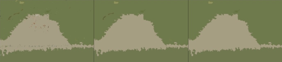
Let's run the same code for the image of the bird and try different values for both parameters. In the following code example, we will be running the felzenszwalb function with the setups (10), (30, 50), and (35, 300), shown as follows:
# load an image
img = load("sample-images/bird-3183441_640.jpg");

# find segments
segments_1 = felzenszwalb(img, 10)
segments_2 = felzenszwalb(img, 30, 50)
segments_3 = felzenszwalb(img, 35, 300)

# the rest of the code from a previous example
...
The results are impressive. The first call separated the bird very well and kept most of the details of the image. Both the second and third versions are much-simplified versions of the original image, with the third image being reduced to only a few segments, thus selecting the foreground area very well, which is shown in the following image:
