Creating a panorama from many images

Another interesting activity you can perform using BRIEF or any of the other methods described in the following section is panoramic view creation. Let's assume you have many images of a sample place and you would like to connect them together and make one single result. We can try using BRIEF to connect the images based on their common features.

As always, let's start by loading the image of a cat into Julia and splitting it into two parts we will be trying to connect afterward. This requires us to define additional parameters, such as the width of the two new images. We will use the following code for this task:

using Images, ImageFeatures, ImageDraw, ImageShow
img = load("sample-images/cat-3418815_640.jpg")

img_width = size(img, 2)
img_left_width = 400
img_right_width = 340

Next, let's create two new images using the preceding settings. We will keep both the original and the grayscale versions. The grayscale version will be used to find the keypoints, and the color version will be used to create the final result. Take a look at this code:

img_left = view(img, :, 1:img_left_width)
img_left_gray = Gray.(img_left)
img_right = view(img, :, (img_width - img_right_width):img_width)
img_right_gray = Gray.(img_right)

imshow(img_left)
imshow(img_right)

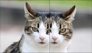
The following images are our two new images we will be trying to connect next:

So, let's find the keypoints from the results of a fastcorners function, by using this code:

keypoints_1 = Keypoints(fastcorners(img_left_gray, 12, 0.3));
keypoints_2 = Keypoints(fastcorners(img_right_gray, 12, 0.3));

Now it is time to initialize BRIEF and find the matches between the features, using this code:

brief_params = BRIEF()
desc_1, ret_features_1 = create_descriptor(img_left_gray, keypoints_1, brief_params);
desc_2, ret_features_2 = create_descriptor(img_right_gray, keypoints_2, brief_params);
matches = match_keypoints(ret_features_1, ret_features_2, desc_1, desc_2, 0.1)

We can preview the results to see whether the keypoints were matched correctly by using this code:

grid = hcat(img_left, img_right)
offset = CartesianIndex(0, size(img_left_gray, 2))
map(m -> draw!(grid, LineSegment(m[1], m[2] + offset)), matches)
imshow(grid)

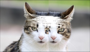
From the following image, you can see lots of different connections. I deliberately kept the number of features high to show different mismatches:

So, what should we do next? Let's assume that most of the points are identified correctly. If so, we can calculate the distance between each of the pairs of keypoints and find the median value that will represent the true value and will call it an offset. Take a look at this code:

offset_x = mean(map(m -> (img_left_width - m[1][2]) + m[2][2], matches))

To simplify the remaining steps, we divide the offset by half and reduce both images for the resulting value. Finally, we preview the outcome in line with the original image:

offset_x_half = Int(trunc(diff_on_x / 2))
img_output = hcat(
 img_left[:, 1:(img_left_width-offset_x_half)],
 img_right[:, offset_x_half:img_right_width]
)

imshow(hcat(img, img_output))

Great work! As you can see from this image, it is very hard to tell the difference between the two images!