Frequency Analysis Part II
Nonstationary Signals and Spectrograms
The goal of this chapter is to extend Fourier analysis as covered in the previous chapter to nonstationary signals. The short-time Fourier transform will be introduced. Nonstationary examples will include applications to time-varying auditory signals and the EEG during sleep.
Keywords
short-time Fourier transform; nonstationary signals; ergodicity; Gabor transform; spectrogram
12.1 Goal of this Chapter
The goal of this chapter is to extend Fourier analysis as covered in the previous chapter to nonstationary signals. The short-time Fourier transform will be introduced. Nonstationary examples will include applications to time-varying auditory signals and the EEG during sleep.
12.2 Background
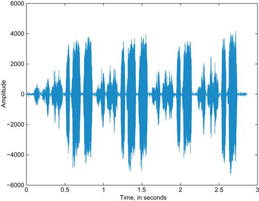
Figure 12.1 depicts the vocalizations of a zebra finch. How is this dissimilar from the sound signals you have examined thus far?
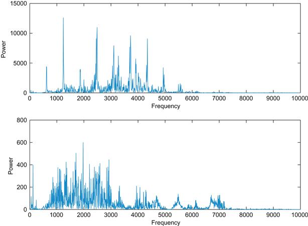
Note that different portions of the song have different envelopes with clearly defined breaks. If they are taken separately, you might imagine these subsections to have different Fourier spectra. In fact, they do. Figure 12.2 shows the Fourier spectrum for two subsections of song. The two subsections have very different distributions of power over frequency.

Figure 12.2 The power spectra of two portions of the zebra finch vocalizations depicted in Figure 12.1.
A Fourier transform of the full song returns the power distribution over the entire song. Any localization of frequency information to a time point or an interval is lost. Using the example of the bird song here, a Fourier transform of the entire song would eliminate any ability to associate frequency components with a given syllable. How, then, can you extend the techniques discussed earlier to such complex signals?
12.2.1 The Fourier Transform: Stationary and Ergodic
When applied to a signal, the term stationary indicates that certain statistical properties of the signal are uniform throughout. In other words, a subset of the signal is sufficient for analysis of the entire signal. The distribution of power over frequency remains the same over the whole signal.
A similar idea is the concept of ergodicity. Imagine an ensemble of related signals. Going with the example of zebra finch vocalizations, an appropriate ensemble would be the set of vocalizations from a set of birds. An ergodic ensemble is one in which each sample and the ensemble approach the same mean. In other words, analyzing one sample or a subset of the signals from the group can approximate the analysis of the ensemble. Ergodicity and stationarity are independent qualities. Neither implies the other.
The Fourier transform assumes a stationary signal. Unfortunately, many biological signals, including the birdsong in Figure 12.1, are nonstationary.
12.2.2 Windows
How can you employ the Fourier transform to a nonstationary signal? If you assume that the Fourier spectrum will change relatively little over a small interval of the signal, you could divide the overall signal into windows and calculate the Fourier transform for each window separately. If a signal is relatively stationary over short intervals, or quasistationary, this approach will often produce fruitful results. While many biological signals are not truly stationary, many are quasistationary and amenable to this approach.
However, this approach breaks down somewhat at the interval boundaries, due to the stationary assumptions of the Fourier transform. Choosing overlapping intervals mitigates this somewhat. This is the basis for the short-time Fourier transform (STFT).
While a simple flat subset of the original time series might be the most straightforward window, an appropriate choice of window shape can amplify or minimize characteristics of the time series. For example, windows with tapered ends are used to minimize artifacts from the edges of the window. This suggests a generalized window function, w(t), which returns the value of the window at a given value of t. For values outside the window, w(t) should return values equal to or close to 0.
Mathematically, the STFT is represented as:
 (12.1)
for a continuous signal. In this case, we are more interested in the discrete STFT,
 (12.2)
As mentioned previously, there are many alternatives to the simple squared off window for calculating an STFT. We will briefly discuss three. The Hamming window function is commonly used:
 (12.3)
where N is the number of points and n varies over the interval.
The Signal Processing Toolbox of the MATLAB® software provides the function hamming, which returns a Hamming window of the desired length:
Note that the Hamming window has a high amplitude at the center and low amplitude at the ends. This attenuation reduces the artifacts from the edge of the window interval. Another window function is the Hann window, whose functional form is similar to the Hamming window:
 (12.4)
Like the Hamming window, the shape of the Hann window is used to reduce artifacts introduced at the edges of the finite windows from the signal. Gaussian window functions are often used as well:
 (12.5)
A short-time Fourier transform using a Gaussian window function is sometimes denoted as a Gabor transform. A Gabor function is the product of a sinusoid and a Gaussian function. The Gaussian function causes the amplitude of the sinusoid to diminish away from the origin, but near the origin, the properties of the sinusoid dominate. By applying a Gaussian window and a Fourier transform to the time series, you are, in effect, applying a Gabor function filter to the data.
12.3 Exercises
As a part of the Signal Processing Toolbox, MATLAB provides the function spectrogram, which calculates a short-time Fourier transform using a Hamming window. The data for Figure 12.1 is available on the companion web site. Download the file song1.wav, and load the file with wavread as follows:
The function wavread loads a sound file in WAVE format and returns the data as amplitude information ranging from −1 to +1. Here, you store the amplitude information in the variable amp. The sampling rate is returned in fs, and the number of bits per sample (resolution) is stored in nbits.
You should see something like Figure 12.3. The default operation of spectrogram calculates power of the signal by dividing the whole signal into eight portions with overlap and windowing the portion with a Hamming window. Here, the specified window size was 256. The optional parameter ‘yaxis’ specifies that frequency should be on the y-axis rather than x-axis. If no return values are specified, the default operation renders the power spectral density over time using “hotter” colors (red, yellow, etc.) to designate frequency bands of greater energy.
If a sampling frequency is not specified, the time scale will not be correct. To show the correct time space for the loaded song, type
Here, the empty brackets signify that the default settings for the window overlap, and FFT size should remain.
Also, spectrogram can return the power spectral density:
The preceding code generates a 3D plot of the spectrogram, where z magnitude, rather than color, represents power.
12.3.1 Limitations of the STFT
The STFT is a fine resolution to the problem of determining the frequency spectrum of signals with time-varying frequency spectra. There are some limitations. Small frequency fluctuations are difficult to detect with the STFT because each subset of the signal is assumed to be stationary. Since the reported frequency distribution at a time point results from the analysis of the entire window, choosing a smaller window does allow for better localization in time. However, a smaller window allows for fewer samples in each Fourier transform, which ultimately reduces frequency resolution, especially for lower frequencies. In other words, a trade-off exists between frequency and time localization.
The STFT is best employed when the fluctuations in frequency occur over a fairly uniform time scale. This allows selecting a single window size without substantial loss of information.
12.4 Project
Typical sleep in human adults includes the well-known REM sleep as well as four well-characterized stages of non-REM sleep, or NREM sleep. During wakefulness, alpha waves dominate the EEG, in the frequency range 8 to 13 Hz. As the person enters the first stage of non-REM sleep, the dominant wave type transitions from alpha waves to theta waves, in the range of 4 to 7 Hz. This is the first stage of non-REM sleep.
The second and third stages of non-REM sleep are characterized by sleep spindles, at 12 to 16 Hz, and the appearance of delta waves, ranging in frequency from 0.5 to 4 Hz. The fourth stage of sleep is characterized by a majority power distribution in the delta wave band. The third and fourth stages of NREM sleep are also termed slow wave sleep, to denote the prevalence of the low frequency delta waves in these two stages.
On the companion web site, you can find three EEGs from patients falling asleep. Using spectrogram and any other frequency analysis tools learned thus far, try to determine when the people enter each of the NREM stages of sleep.

