Models of the Retina

Pascal Wallisch

The goal of this chapter is to understand the basic structure of the retina and to see how to create simple models of neuronal interactions. In this chapter you will build a simple model describing the interaction between cone cells and horizontal cells of the retina and solve it exactly by taking advantage of the capability of the MATLAB® software to easily manipulate matrices.

Keywords

cones; rhodopsin; 11-cis-retinal; 11-trans-retinal; horizontal cells; negative feedback; optic nerve

The retina is the part of the eye that transforms light into an electrochemical message sent to the brain for processing. The mechanism is quite complicated, but we will give a brief overview. Light first contacts the cornea, a transparent tissue covering the pupil and the iris. The cornea helps converge light through the pupil. Next, light passes through the lens, where it is further focused onto the retina in the back of the eye. The retina has five distinct classes of neurons arranged into cell layers. Light first contacts the innermost layers of the retina, but it is the outermost layer that first processes the incoming light signal. The layer responsible for processing the incoming light is composed mainly of two different cell types: cones and rods. Rods are mainly responsible for sensing brightness, and cones are responsible for detecting color.

This chapter pertains to cones, which we will discuss exclusively from now on. Mammals such as humans have three types of cones. Each type is adept at “seeing” a certain color: red, green, or blue. Cones have a G-protein coupled receptor on their cell surface called rhodopsin. This receptor is closely associated with a chromophore called 11-cis-retinal. When a photon of light hits the chromophore, it isomerizes to 11-trans-retinal. This conformational change is detected by the rhodopsin molecule, and a G-protein is activated, which eventually closes ion channels on the cell membrane. The result is that ions (i.e., current) can no longer enter the cell, and the cell hyperpolarizes. Hyperpolarization decreases the cone’s release of glutamate, a neurotransmitter that often has excitatory postsynaptic effects, which in turn decreases activity in postsynaptic cells in the next retinal layer. These postsynaptic cells are called horizontal cells (H-cells). H-cells normally maintain reciprocal synaptic connections with the cones that synapse onto them. H-cells release GABA, a neurotransmitter that has inhibitory postsynaptic effects. When the cones hyperpolarize in response to light and the H-cells decrease activity, the cones become disinhibited and begin to depolarize. This process is referred to as negative feedback because the initial light that induced hyperpolarization causes H-cells to feed back upon the cones in a way that counteracts the initial hyperpolarization. It is believed that this negative feedback is a regulatory mechanism to control color contrast. When the level of negative feedback of horizontal cells to cones is changed, the cones’ response can be altered. Slight changes in feedback might be responsible for helping to determine changes in color. After all, although we have only three types of cones, humans can distinguish between millions of different colors! In addition to feeding back onto cones, horizontal cells also send signals to bipolar cells, which signal to amacrine cells, which finally signal to ganglion cells. The axons of these ganglion cells make up what anatomists call the optic nerve, the large nerve that connects the eye to the brain. The brain is then responsible for decoding the information sent from the retina to create what you “see” when you look at an object.

28.2.2 The Model

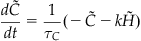
The model used in this chapter will be a system of two linear differential equations. The first will describe changes in the current leaving the cone of the retina, C(t), and the second will describe the current leaving the horizontal cell, H(t). We could build a larger system to account for the bipolar cells, amacrine cells, and ganglion cells, but we will keep it simple for now. The system is represented as follows:

(28.1)

(28.2)

The first equation has three terms. The first indicates that the change in current is negatively proportional to the amount of current inside the cone, C. The second term represents the fact that the change in current is proportional to the current inside the horizontal cell, H, which negatively feeds back on the cell, and the third term indicates that the change in current into the cone is dependent on the light level, L. If the light level is high, then many photons will pass through the pupil, land on the retina, and activate the cones, resulting in a large change in current. The second equation states that the change in current in the horizontal cells depends negatively on the amount of current in the horizontal cells and the current of the cone cell that synapses onto the horizontal cell. Recall that the horizontal cells do not respond directly to light stimuli, so there is no term for the light intensity in the second equation. All other symbols in the preceding equations represent parameters (i.e., constants). Typical values for these parameters are τ_C=0.025 sec, τ_H=0.08 sec, and k=4. Now also assume that the light intensity, L, is a constant, particularly L=10. Finally, for the initial conditions, choose that C(0)=H(0)=0. There is no current moving through either cell at t=0.

The model equations as they are currently written can be simplified by a clever substitution. If you let:

(28.3)

and substitute these equations into the previous equations, then you get:

(28.4)

(28.5)

This is the model that you will study in its final form in this chapter. Note that the initial conditions now give:

(28.6)

28.2.3 Mathematical Background

Systems like the one in Equations 28.4 and 28.5 are especially suitable for study in MATLAB because they can be readily solved using simple matrix manipulations, as illustrated in the following simple example. Suppose you wanted to solve the system shown in Equations 28.7 and 28.8:

(28.7)

(28.8)

You begin by writing this system in matrix form to get:

(28.9)

If you let the vector

(28.10)

then the system in Equations 28.7 and 28.8 becomes:

(28.11)

Based on the Eigendecomposition Theorem (see Appendix B, “Linear Algebra Review”), you can substitute in for A to get the following equation:

(28.12)

Next, you multiply across the left by V⁻¹ to get:

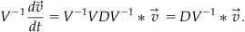(28.13)

If you let, then Equation 28.11 becomes:

(28.14)

This equation is similar to Equation 28.11, except for one very important exception: D is diagonal. The eigendecomposition of:

gives the eigenvalue matrix

and the eigenvector matrix

If you substitute in for D and convert Equation 28.14 into a system of equations, you get:

(28.15)

This system is also a system of differential equations. However, each equation can be solved independently of one another to yield the solution:

(28.16)

Finally, recall that you let , and:

(28.17)

Notice where the eigenvalues and eigenvectors appear in the preceding solution. The eigenvalues, −1 and 3, appear in the exponents, and the eigenvectors appear as constant vectors multiplying the exponential with the corresponding eigenvalue. In general, the solution to any system of the form given in Equation 28.11 is:

(28.18)

where λ₁ and λ₂ are distinct (not equal) eigenvalues of the matrix A, and EV₁ and EV₂ are the corresponding eigenvectors. If A has eigenvalues that are the same, then Equation 28.18 does not apply.

28.3 Exercises

You can see from Equation 28.18 that any set of equations that can be made into the form of Equation 28.11 can be solved by finding the eigenvalues and eigenvectors of the matrix A, as long as A has distinct eigenvalues. You can do this easily in MATLAB with the following command:

>>[V, D] = eig(A);

For example, typing the command

>>[V, D] = eig([1 1;4 1])

produces the response:

V =

0.4472 −0.4472
0.8944 0.8944

D =

3.0000 0
0 −1.0000.

The matrix D is a diagonal matrix with diagonal elements given by the eigenvalues of A. The columns of the matrix V correspond to the eigenvectors of A. The matrix D is the same as the one given earlier used to derive Equation 28.15, but the matrix V produced by MATLAB is different from the one used to derive Equation 28.17. Nonetheless, you still have the relationship that A=VDV⁻¹. You can check this by typing the command

>> V*D*inv(V)

ans =

1.0000 1.0000
4.0000 1.0000.

The inv() function determines the inverse of a matrix.

Reexamining Equation 28.18 reveals that in order to find x(t) and y(t), you still need to solve for C₁ and C₂. It can be shown that if you have the initial conditions that x(0)=x_o and y(0)=y_o, then: