Chapter 10

LEARNING TO BE THOUGHTLESS: SOCIAL NORMS
AND INDIVIDUAL COMPUTATION

JOSHUA M. EPSTEIN^*

THIS PAPER EXTENDS the literature on the evolution of norms with an agent-based model capturing a phenomenon that has been essentially ignored, namely that individual thought—or computing—is often inversely related to the strength of a social norm. Once a norm is entrenched, we conform thoughtlessly. In this model, agents learn how to behave (what norm to adopt), but—under a strategy I term Best Reply to Adaptive Sample Evidence—they also learn how much to think about how to behave. How much they are thinking affects how they behave, which—given how others behave—affects how much they think. In short, there is feedback between the social (inter-agent) and internal (intra-agent) dynamics. In addition, we generate the stylized facts regarding the spatio-temporal evolution of norms: local conformity, global diversity, and punctuated equilibria.

TWO FEATURES OF NORMS

When I'd had my coffee this morning and went upstairs to get dressed for work, I never considered being a nudist for the day. When I got in my car to drive to work, it never crossed my mind to drive on the left. And when I joined my colleagues at lunch, I did not consider eating my salad barehanded; without a thought, I used a fork.

The point here is that many social conventions have two features of interest. First, they are self-enforcing behavioral regularities (Lewis 1969; Axelrod 1986; Young 1993a, 1995). But second, once entrenched, we conform without thinking about it. Indeed, this is one reason why social norms are useful; they obviate the need for a lot of individual computing. After all, if we had to go out and sample people on the street to see if nudism or dress were the norm, and then had to sample other drivers to see if left or right were the norm, and so on, we would spent most of the day figuring out how to operate, and we would not get much accomplished. Thoughtless conformity, while useful in such contexts, is frightening in others—as when norms of discrimination become entrenched. It seems to me that the literature on the evolution of norms and conventions has focused almost exclusively on the first feature of norms—that they are self-enforcing behavioral regularities, often represented elegantly as equilibria of n-person coordination games possessing multiple pure-strategy Nash equilibria (Young 1993a, 1995; Kandori, Mailith, and Rob 1991).

GOALS

My aim here is to extend this literature with a simple agent-based model capturing the second feature noted above, that individual thought—or computing—is inversely related to the strength of a social norm. In this model, then, agents learn how to behave (what norm to adopt), but they also learn how much to think about how to behave. How much they are thinking affects how they behave, which—given how others behave—affects how much they think. In short, there is feedback between the social (inter-agent) and internal (intra-agent) dynamics. In addition, we are looking for the stylized facts regarding the spatio-temporal evolution of norms: local conformity, global diversity, and punctuated equilibria (Young 1998).

AN AGENT-BASED COMPUTATIONAL MODEL

This model posits a ring of interacting agents. Each agent occupies a fixed position on the ring and is an object characterized by two attributes. One attribute is the agent's “norm,” which in this model is binary. We may think of these as ‘drive on the right (R) vs. drive on the left (L).' Initially, agents are assigned norms. Then, of course, agents update their norms based on observation of agents within some sampling radius. This radius is the second attribute and is typically heterogeneous across agents. An agent with a sampling radius of 5 takes data on the five agents to his left and the five agents to his right. Agents do not sample outside their current radius. Agents update, or “adapt,” their sampling radii incrementally according to the following simple rule:

RADIUS UPDATE RULE

Imagine being an agent with current sampling radius of r. First, survey all r agents to the left and all r agents to the right. Some have L (drive on the left) as their norm and some have R(drive on the right). Compute the relative frequency of Rs at radius r ; call the result F (r). Now, make the same computation for radius r + 1. If F (r + 1) does not equal F (r), then increase your search radius to r + 1.¹ Otherwise, compute F (r – 1). If F (r – 1) does equal F (r), then reduce your search radius to r – 1. If neither condition obtains (i.e., if F (r + 1) = F (r) ≠ F (r – 1)), leave your search radius unchanged at r.

Agents are “lazy statisticians,” if you will. If they are getting a different result at a higher radius (F (r + 1) ≠ F (r)), they increase the radius—since, as statisticians, they know larger samples to be more reliable than smaller ones. But they are also lazy. Hence, if there's no difference at the higher radius, they check a lower one. If there is no difference between that and their current radius (F (r – 1) = F (r)), they reduce. This is the agent's radius update rule. Having updated her radius, the agent then executes the Norm Update Rule.

NORM UPDATE RULE

This is extremely simple: match the majority within your radius. If, at the updated radius, Ls outnumber Rs, then adopt the L norm. In summary, the rule is: When in Rome, do as the (majority of) Romans do, with the (adaptive) radius determining the “city limits.” This rule is equivalent to Best Reply to sample evidence with a symmetric payoff matrix such as:

Following Young (1996), we imagine a coachman's decision to drive on the left or the right. “Among the encounters he knows about, suppose that more than half the carriages attempted to take the right side of the road. Our coachman then predicts that, when he next meets a carriage on the road, the probability is better than 50-50 that it will go right. Given this expectation, it is best for him to go right also (assuming that the payoffs are symmetric between left and right).” The coachman “calculates the observed frequency distribution of left and right, and uses this to predict the probability that the next carriage he meets will go left or right. He then chooses a best reply,” which Young terms “best reply to recent sample evidence.” Best reply maximizes the expected utility (sum of payoffs) in playing the agent's sample population.²

The departure introduced here is that each individual's sample size is itself adaptive.³ In particular, as suggested earlier, once a norm of driving on the left is established (firmly entrenched) real coachmen don't calculate anything—they (thoughtlessly and efficiently) drive on the left. So, we want a model in which “thinking”—individual computing—declines as a norm gains force, and effectively stops once the norm is entrenched. Of course, we want our coachmen to start worrying again if suddenly the norm begins to break down. Of the many adaptive individual rules one might posit, we will explore the radius update rule set forth above.

Overall, the individual's combined (norm and search radius) updating procedure might appropriately be dubbed Best Reply to Adaptive Sample Evidence.

NOISE

Finally, there is generally some probability that an agent will adopt a random norm, a random L or R. We think of this as a “noise” level in society.

Graphics

With this set-up, there are two things to keep track of: the evolution of social norm patterns on the agent ring, and the evolution of individual search radii. In the runs shown below, there are 191 agents. They are drawn at random and updated asynchronously. Clearly, each agent's probability of being drawn k times per cycle (191 draws with replacement) has the binomial distribution b(k; n,1/n), with n = 191. Agents who are not drawn keep their previous norm. After 191 draws—one cycle—the new ring is redrawn below the old one (as a horizontal series of small contiguous black and white dots), so time is progressing down the page. There are two Panels. The left Panel shows the evolution of norms, with L-agents colored black and R-agents colored white. With the exception of Run 4, each entire Panel displays 300 cycles (each cycle, again, being a sequence of 191 random calls.) The right window shows the evolution of search radii, using grayscale. Agents are colored black if r = 1, with progressively higher radii depicted as progressively lighter shades of gray.

RUNS OF THE MODEL

We present seven basic runs of this model, and some statistical and sensitivity analysis. Once more, we are looking for the stylized facts regarding the evolution of norms: Local conformity, global diversity, and punctuated equilibria (Young 1998). But we wish also to reflect the rise and fall of individual computing as social norms dissolve and become locked in.

Run 1. Monolithic Social Norm, Individual Computing Dies Out

For this first run, we set all agents to the L norm (coloring them black) initially and set noise to zero. We give each agent a random initial search radius between 1 and 60 (artificially high to show the strength of the result in the monolithic case). There is no noise in the decision-making. The uppermost line (the initial population state) of the right graph (191 agents across) is multi-shaded, reflecting the random initial radii. Let us now apply the radial update rule to an arbitrary agent with radius r. First look out further. We find that F (r + 1) = F (r), since all agents are in the L norm (black). Hence, try a smaller radius. Since F (r – 1) = F (r), the agent reduces from r to r – 1. Now, apply the norm update rule. At this new radius, match the majority. Clearly, this is L (black), so stay L. This is the same logic for all agents. Hence, on the left panel of figure 10.1, the L social norm remains entrenched, and, as shown in the right panel, individual “thinking” dies out—radii all shrink to the minimum of 1 (colored black).

Run 2. Random Initial Norms, Individual Computing at Norm Boundaries

With noise still at zero, we now alter the initial conditions slightly. In this, and all subsequent runs, the initial maximum search radius is 10. Rather than set all agents in the L norm initially, we give them random norms. In figure 10.2, we see a typical result.

In the left panel, there is rapid lock-in to a global pattern of alternating local norms on the ring. In the right panel, we see that deep in each local norm, agents are colored black: there is no individual computing, no “thinking,” as it were. By contrast, agents at the boundary of two norms must worry about how to behave, and so are bright-shaded.⁴ (For future reference notice that, since there are two edges for each local norm—each stripe on the left panel—the average radius will stabilize around different values from run to run, depending on the number of different norms that emerge.)

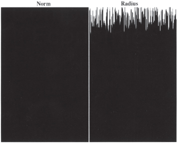
Figure 10.1. Monolithic norms induce radial contraction.

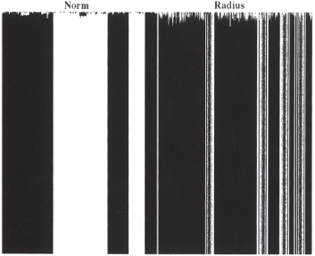
Figure 10.2. Local conformity, global diversity, and thought at boundaries.

Run 3. Complacency in New Norms

In the 1960's, people smoked in airplanes, restaurants, and workplaces, and no one gave it much thought. Today, it is equally entrenched that smoking is prohibited in these circumstances. The same point applies to other social norms (e.g., revolutions in styles of dress) and to far more momentous political ones (e.g., voting rights, segregation of water fountains, lunch counters, and seats on the bus). After the “revolution” entirely new norms prevail, but once entrenched, people become inured to them; they are observed every bit as thoughtlessly (in our sense) as before. I often feel that the same point applies to popular beliefs about the physical world; these represent a procession of conventions rather than any real advance in the average person's grasp of science. For example, if you had asked the average 14th Century European if the earth were round or flat, he would have said “flat.” If, today, you ask the average American the same question, you will certainly get a different response: “round.” But I doubt that the typical American could furnish more compelling reasons for his correct belief than our 14th Century counterpart could have provided for his erroneous one. Indeed, on this test, the “modern” person will likely fare worse: at least the 14th Century “norm” accorded with intuition. Maybe we are going backward! In any event, there was no “thinking” in the old norm, and there is little or no thinking in the new one. Again, the point is that after the “revolution,” new conventions prevail, but once entrenched, they are conformed to as thoughtlessly as their predecessors. Does our simple model capture that basic phenomenon?

In Run 3, we begin as before, with randomly distributed initial norms and zero noise. We let the system “equilibrate,” locking into neighborhood norms (as before, these appear as vertical stripes over time). Then, at t = 130, we shock the system, boosting the level of noise to 1.0, and holding it there for ten periods. Then we turn the noise off and watch the system re-equilibrate. Figure 10.3 chronicles the experiment.

After the shock, an entirely new pattern of norms is evident on the lefthand page. But, looking at the right-hand radius page, we see that many agents who were thoughtlessly in the L norm (black) before the shock are equally thoughtlessly in the R norm (white) after.

A time series plot of average radius over the course of this experiment is also revealing. See figure 10.4. Following an initial transient phase, the mean radius attains a steady state value of roughly 2.25. During the brief “shock” period of maximum noise, the average radius rises sharply, reflecting the agents’ frenetic search for appropriate behavior in a period of social turmoil. One might expect that, with noise restored to zero, the average radius would relax back to its pre-shock value. In fact—as foreshadowed above—the post-shock steady state depends on the post-shock number of local norms. The lower the diversity, the lower the number of borders and, as in the present run, the lower the average radius.

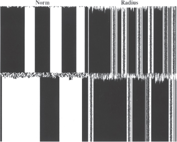
Figure 10.3. Re-equilibration after shock.

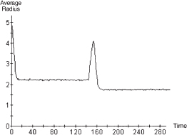
Figure 10.4. Shock experiment. Time series of average radius.

Run 4. Noise of 0.15 and Endogenous Neighborhood Norms

Now, noise levels of zero and one are not especially plausible. What norm patterns, if any, emerge endogenously when initially random agents play our game, but with a modest level of noise (probability of adopting a random norm)? The next four runs use the same initial conditions as Run 2, but add increasing levels of noise. With noise set at 0.15, we obtain dynamics of the sort recorded in figure 10.5.

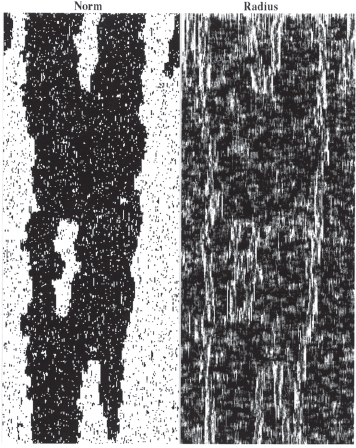
Figure 10.5. Noise of 0.15 and endogenous norms.

Again, we see that individual computing is most intense at the norm borders—regions outlining the norms. We also see the emergence and disappearance of norms, the most prominent of which is the white island that comes into being and then disappears. One can think of islands as indicating punctuated equilibria.

For the realization depicted spatially above, the time series for average radius is given in figure 10.6. Following an initial transient phase, the average search radius clearly settles at roughly 2.0 for this realization.⁵ Even at zero cost of sampling, in other words, a “stopping rule” for the individual search radius emerges endogenously through local agent interactions. And this obtains at all levels of noise, as we shall see.

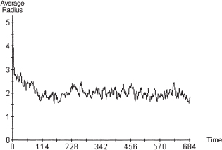
Figure 10.6. Noise of 0.15 time series of average radius.

Now, in the cases preceding this one, there was zero noise in the agents’ decision-making, and—although there would be run-to-run differences due to initial conditions and random agent call order—the point of interest was qualitative, and did not call for statistical discussion. However, in this and subsequent cases, there is noise, and quantitative matters are of interest. Hence, data from a single realization may be misleading and a statistical treatment is appropriate. The statistical analysis of simulation output has itself evolved into a large area, and highly sophisticated methods are possible. See Law and Kelton 1991 and Feldman and Valdez-Flores 1996. Our approach will be simple.

STATISTICAL RESULTS

To estimate the expected value of the long-run average search radius in this noise = 0.15 case, the model was rerun 30 times (so that, by standard appeal to the central limit theorem, a normal approximation is defensible) with a different random seed each time (to insure statistical independence across runs). In each run, the mean data were sampled at t = 300 (long after any initial transient had damped out). For a considered discussion of simulation stopping times, and all the complexities of their selection, see Judd 1999. The resulting 95% confidence interval⁶ for the steady state mean search radius is [1.89, 2.03]. We double the noise level to 0.30 in Run 5.

Run 5. Noise of 0.30 and Endogenous Neighborhood Norms

The result, shown in figure 10.7, is a more elaborate spatial patterning than in the previous run. Again, however, we see regions of local conformity amidst a globally diverse pattern.

In this run, we see the emergence of white and black islands, indicating punctuated equilibria once more. For this realization, the mean radius time series is plotted in figure 10.8. Computed as above, the 95% confidence interval for the steady state mean radius is [2.89, 3.04].

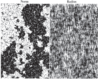
Figure 10.7. Noise of 0.30 and endogenous norms.

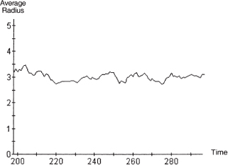
Figure 10.8. Noise of 0.30 time series of average radius.

Run 6. Noise of 0.50

Pushing the noise to 0.50 results in the patterning shown in figure 10.9, for which the average radius is plotted in figure 10.10. The 95% confidence interval for the long-run average search radius is [3.73, 3.81].

Run 7. Maximum Noise Does Not Induce Maximum Search

Finally, we fix the noise level at its maximum value of 1.0, meaning that agents are adopting the Left and Right convention totally at random. One might assume that, in this world of maximum randomness, agents would continue to expand their search to its theoretical maximum of (n – 1)/2, or 95 in this case. But this is not what happens, as evident in figure 10.11. Indeed, as plotted in figure 10.12, it rises only to about 4.5. Computed as above, the 95% confidence interval is [4.53, 4.63]. Thinking—individual computing—is minimized in the monolithic world of Run 1. But, it does not attain its theoretical maximum in the totally random world of this run.

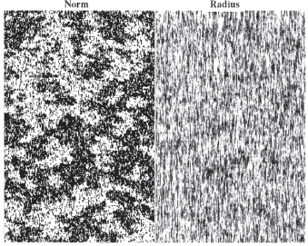
Figure 10.9. Noise of 0.50.

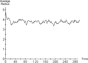
Figure 10.10. Noise of 0.5 time series of average radius.

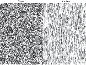
Figure 10.11. Noise of 1.0.

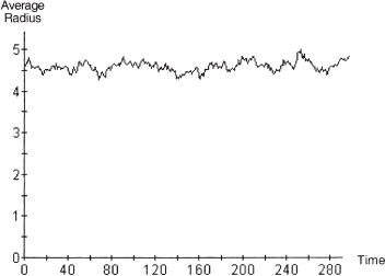
Figure 10.12. Noise of 1.0 time series of average radius.

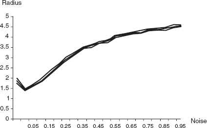
Figure 10.13. Steady state average radius and confidence intervals as function of noise at tolerance = 0.05.

Figure 10.13 gives a summary plot of the long-run average radius (middle curve) and 95% confidence intervals (outer curves) for noise levels ranging from 0 to 1, in increments of 0.05. Note that, at all noise levels, the confidence intervals are extremely narrow.

Sensitivity to the Tolerance Parameter

In all of the runs and statistical analyses given above, the tolerance parameter (see note 1) was set at 0.05, meaning that in applying the radius update rule, the agent regards F (r) and F (r + 1) as equal if they are within 0.05 of one another. The agent's propensity to expand the search radius is inversely related to the tolerance. Figure 10.14 begins to explore the general relationship. For tolerances of 0.025 and 0.10, it displays the same triplet of curves as shown in figure 10.13 for T = 0.05 (which curve is also reproduced). All confidence intervals are again very narrow.

Even at the lowest tolerance of 0.025,⁷ the average search radius does not attain the theoretical maximum even if the noise level does.

Finally, just to ensure that these results on the boundedness of search are not an artifact of sampling at t = 300, we conducted the same analysis again, but sampling at t = 10,000. The results are compared in figure 10.15. The solid curves are the average search radii from the previous figure, computed at t = 300. The dotted curves are the corresponding data computed at t = 10,000. Clearly, for noise above roughly 0.20, there are no discernable differences at any of the three tolerances. (And for the low noise cases where there is some small difference, it is in fact the t = 10,000 curve that is lower.)⁸ Search is bounded, even when noise is not.⁹

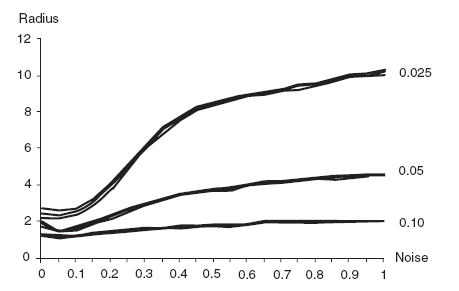
Figure 10.14. Steady state average radii and confidence intervals as function of noise at various tolerances, sampling at t = 300.

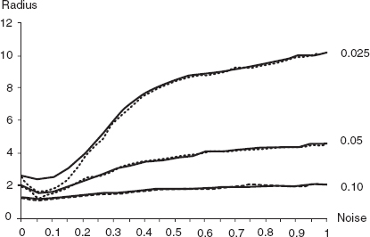
Figure 10.15. Steady state average radii as function of noise at various tolerances, sampling at t = 300 vs. t = 10,000.

SUMMARY

My aim has been to extend the literature on the evolution of social norms with a simple agent-based computational model that generates the stylized facts regarding the evolution of norms—local conformity, global diversity, and punctuated equilibria—while capturing a central feature of norms that has been essentially ignored: that individual computing is often inversely related to the strength of a social norm. As norms become entrenched, we conform thoughtlessly. Obviously, many refinements, further sensitivity analyses, analytical treatments, and extensions are possible. But the present exposition meets these immediate and limited objectives.

Java Implementation

The model has been implemented in C++ and in Java. The Java implementation uses ASCAPE, an agent modeling environment developed at Brookings. Readers interested in running the model under their own assumptions may do so using this book's CD.

REFERENCES

Axelrod, Robert. 1984. The Evolution of Cooperation. New York: Basic Books.

_____. 1996. An Evolutionary Approach to Norms. American Political Science Review 80(4): 1095-1111.

_____. 1997. The Complexity of Cooperation: Agent-Based Models of Competition and Collaboration. Princeton: Princeton University Press.

Bicchieri, Cristina, Richard Jeffrey, and Brian Skyrms, eds. 1997. The Dynamics of Norms. New York: Cambridge University Press.

Canning, David. 1994. Learning and Social Equilibrium in Large Populations. In Learning and Rationality in Economics, ed. Alan Kirman and Mark Salmon. Oxford: Blackwell.

Feldman, David P., and James P. Crutchfield. 1997. Measures of Statistical Complexity: Why? Santa Fe Institute Working Paper 97-07-064.

Feldman, Richard M., and Ciriaco Valdez-Flores. 1996. Applied Probability and Stochastic Processes. Boston: PWS Publishing.

Freund, John E. 1992. Mathematical Statistics. 5th ed. Upper Saddle River, NJ: Prentice Hall.

Glaeser, Edward L., Bruce Sacerdote, and Jose Scheinkman. 1996. Crime and Social Interactions. Quarterly Journal of Economics 111:507-48.

Judd, Kenneth L. 1998. Numerical Methods in Economics. Cambridge: MIT Press.

Kandori, Michihiro, George J. Mailath, and Rafael Rob. 1993. Learning, Mutation, and Long-Run Equilibria in Games. Econometrica 61:29-56.

Kirman, Alan, and Mark Salmon, eds. 1994. Learning and Rationality in Economics. Oxford: Blackwell.

Law, Averill M., and W. David Kelton. 1991. Simulation Modeling and Analysis. New York: McGraw-Hill.

Lewis, David K. 1969. Convention: A Philosophical Study. Cambridge: Harvard University Press.

Ullman-Margalit, Edna. 1977. The Emergence of Norms. Oxford: Oxford University Press.

Vega-Redondo, Fernando. 1996. Evolution, Games, and Economic Behaviour. Oxford: Oxford University Press.

Young, H. Peyton. 1993a. The Evolution of Conventions. Econometrica 61:57-84.

_____. 1993b. An Evolutionary Model of Bargaining. Journal of Economic Theory 59:145-68.

_____. 1996. The Economics of Convention. Journal of Economic Perspectives 10:105-22.

_____. 1998. Individual Strategy and Social Structure. Princeton: Princeton University Press.

---

^* For valuable discussions the author thanks Peyton Young, Miles Parker, Robert Axtell, Carol Graham, and Joseph Harrington. He further thanks Miles Parker for translating the model, initially written in C++, into his Java-based ASCAPE environment. For production assistance, he thanks David Hines.

This essay was published previously in Computational Economics, vol. 18, no. 1, August 2001, pp. 9-24.

¹ When we say “not equal” we mean the difference lies outside some tolerance, T. That is, |F (r + 1) – F (r)| > T for inequality, and |F (r + 1) – F (r)|≤ T for equality. For our basic runs, T = 0.05.

² For arbitrary payoff matrices, Best Reply is not equivalent to the following rule: Play the strategy that is optimal against the most likely type of opponent (i.e., the strategy type most likely to be drawn in a single random draw from your sample). For our particular set-up, these are both equivalent to our “match the majority” update rule. These three rules part company if payoffs are not symmetric.

³ In Best Reply models, the sample size is fixed for each agent, and is equal across agents. See Young 1995.

⁴ For the particular realization shown in figure 10.2, the average radius settles (after the initial transient phase) to around 3.

⁵ For the sake of visibility, the vertical axis ranges from zero to five. While, at this resolution, the plot may appear quite variable, the fluctuations around 2.0 are minor, given that the maximum possible radius is (n – 1)/2, or 95 in this case.

⁶ This is computed as as in Freund (1992, 402), with = 1.96, and the average and s the standard deviation over our n = 30 runs.

⁷ Tolerances much below this are of questionable interest. First, we detect virtually no spatial norm patterning. Second, one is imputing to agents the capacity to discern differences in relative norm frequency finer than 25 parts in a thousand, which begins to strain credulity.

⁸ The 95% confidence intervals (not shown) about the t = 10,000 curves are extremely narrow, as in the t = 300 cases.

⁹ This demonstrated stability of the average search radius to t = 10,000 does not preclude mathematically the asymptotic approach to other values; an analytical treatment would be necessary to do that. On the other hand, even if established, the existence of asymptotic values significantly different from those that persist to (at least) t = 10,000 would be of debatable interest. As Keynes put it, “In the long run, we are all dead.”