Chapter 7

COORDINATION IN TRANSIENT SOCIAL
NETWORKS: AN AGENT-BASED COMPUTATIONAL
MODEL OF THE TIMING OF RETIREMENT

ROBERT L. AXTELL AND JOSHUA M. EPSTEIN^*

THOUGH MOTIVATED by a policy question, this work has theoretical dimensions. There are two related theoretical issues. One is the connection between individual rationality and aggregate efficiency—between optimization by individuals and optimality in the aggregate. The second is the role of social interactions and social networks in individual decision making and in determining macroscopic outcomes and dynamics. Regarding the first, much of mathematical social science assumes that aggregate efficiency requires individual optimization. Perhaps this is why bounded rationality is disturbing to some economists: they implicitly believe that if the individual is not sufficiently rational, it must follow that decentralized behavior is doomed to produce inefficiency. The invisible hand requires rational fingers, if you will.

Experimental economics and psychology have produced strong empirical support for the view that framing effects, as well as contextual and other psychological factors, create a large gap between homo economicus and homo sapiens.¹ Individual rationality is bounded. The questions we pose here are: Does that matter? How does it matter?

To answer these questions, we have developed a model in which imitation in social networks can ultimately yield high aggregate levels of optimal behavior despite extremely low levels of individual rationality. The fraction of agents who are rational in such an imitative system will definitely affect the rate at which a steady state sets in. But the eventual (asymptotic) attainment per se of such a state need not depend on the extent to which rationality is bounded. Perhaps the main issue, then, is not how much rationality there is at the micro level, but how little is enough to generate macro-level patterns in which most agents are behaving “as if” they were rational, and how various social networks affect the dynamics of such patterns. Of particular concern are the puzzling dynamics of retirement.

In 1961 Congress reduced the minimum age at which workers could claim social security benefits from sixty-five to sixty-two. By any measure, this was a major policy shift. Yet it took nearly three decades for the modal retirement age to fall correspondingly. While various explanations are possible, we suggest that imitative behavior and social interactions—factors absent from traditional economic models—may be fundamental in explaining the sluggish response to policy.

For modeling purposes, one can represent retirement decision making (and perhaps a range of other problems) in the following stylized terms. First, there is an initial state of the world in which the individually optimal age at which to take some action is Y. Suddenly, a policy is instituted exogenously. Given this policy, the individually optimal age at which to take the action becomes Y^* ≠ Y. What one observes, however, is not the instantaneous shift from Y to Y^* that would be predicted assuming universal, fully informed, rational behavior. Rather, there is a long process of patchy social adjustments, in which different clusters of individuals migrate to Y* at different rates, with some groups perhaps not getting there at all. In our model, the action in question is individual retirement, the exogenously instituted policy is the 1961 congressional reduction in the age of eligibility for social security, and Y and Y* are sixty-five and sixty-two, respectively. The actual data are plotted in (figure 7.1.² As noted above, it took nearly three decades for the response—a downward shift in the modal retirement age from sixty-five to sixty-two—to manifest itself. We develop a relatively general model, involving imitation in social networks, that generates such patchy and sluggish dynamics. It is not the only approach possible.³

One body of research has sought to explain the data with aggregate models in which a representative agent solves some life-cycle optimization problem.⁴ If the goal is simply to fit the data, it is not unreasonable to attribute to agents the capacity to explicitly formulate and solve such dynamic programming problems. However, there is strong empirical evidence that humans do not perform well on problems whose solution involves backward induction (see Camerer 1997). For this reason, these models fail to provide a realistic microeconomic—that is, individualist—account of the phenomenon. We would like to provide such an account.

Figure 7.1. Male retirement rate by age, 1960,1970, and 1995-96. (Source: Gary Burtless, personal communication.)

Our model does not invoke a representative agent but posits a heterogeneous population of individuals. Some of these behave “as if” they were fully informed optimizers, while others, indeed most, do not. Social networks and social interactions, clearly absent from the prevailing literature, play an explicit and central role.

A MODEL OF RETIREMENT AGE NORMS

The agents in our model fall into three categories. One minority group of agents adopts the (presumably) optimal policy by a process we do not model. Another minority group is composed of randomly behaving agents who retire with a fixed probability once they reach retirement age. The majority of agents are imitators who mimic members of their social networks. For lack of better terminology, we designate these groups “rationals,” “randoms,” and “imitators,” respectively.

Agents, Cohorts, and Social Networks

The agent population is divided into age cohorts ranging from age twenty to age one hundred. Thus, there are eighty-one cohorts. Each contains C agents for a total of 81C ≡ A agents. Each agent is assigned a random age of death drawn from U[60,100].⁵ The average death age is thus eighty. When an agent dies, it is replaced by a twenty-year-old agent.⁶ In each time period each agent is activated exactly once, and if it is eligible to retire but has not yet done so, decides whether or not to retire.⁷

Agents are heterogeneous by social network; each has its own. A social network is simply a list of other agents, specified randomly and fixed over the agent's lifetime. The number of other agents is set by drawing a random network size, S, from U[a, b]. Some of these agents may be younger or older than the agent in question. The extent, E, represents how far the agent's social network extends above and below its own age cohort; E is drawn from U[0, c]. Thus one agent might have a social network of seventeen others, ranging in age from five years younger to five years older than itself, while another agent might have a social network consisting of thirteen others who are all within a year of its own age. Any two networks may or may not overlap, that is, have agents in common.

Figure 7.2. Typical agent social networks.

At any given time, the set of all social networks constitutes a single random graph, with the agents as nodes and the network relations as directed edges.⁸ Figure 7.2 shows a variety of social networks. Each rectangle represents an agent and each row represents an age cohort, with progressively older cohorts arrayed from top to bottom in the figure. Social networks are shown with X's for the three agents who are colored black, in the sixty, seventy-seven, and ninety-four age cohorts. The twenty-four members of the sixty-year-old agent's social network include thirteen younger agents and eleven older agents.

Agent Types

As noted earlier, there are three broad types of agents. Rational agents retire at the earliest possible age allowed by government policy. Random agents retire with probability p each period, once they reach the age of eligibility for retirement.

Imitator agents are the most heterogeneous and interesting. Each imitator has a unique social network. Within this individual network, there is some fraction f of eligible agents who have actually retired. At each instant this is heterogeneous across agents, since the size and composition of networks are agent-specific. Agents are assigned an imitation threshold, τ, representing the minimum proportion of members of the agent's social network who must be retired for that agent to retire. Each agent's behavioral rule then amounts to comparing τ with f.⁹ If f ≥ τ, the agent retires; otherwise, the agent continues working until the following period, when it reevaluates its decision.

Notionally, the imitator agents play a simple coordination game within their social networks.¹⁰ That is, agents derive utility from coordinating their behavior with the members of their social network. At every instant each agent in the population is either working or retired. Since A is the number of agents, call x {working, retired}^A the state of the population, and x_i agent i ‘s state. Agent i ‘s social network is denoted by N_i. Then the utility that i derives from interacting with the members of its social network in state x, U_i (x), can be written

where u(x_i, x_j) is the utility of i ‘s interaction with j.

The function u can be thought of as the payoff function of a two-by-two symmetric game:

U_i is then the payoff function of the social network game. Note that τ can be expressed in payoff terms. When an agent is young and none of its social peers are retired, f = 0, and the agent derives maximum utility from working. However, as its friends begin to retire (f > 0), the utility from retiring rises to rf, and the utility from working falls from w to w(1 – f). The agent will decide to retire if f rises to a level such that rf ≥ w(1 – f), or equivalently, f ≥ w/(r + w); thus, the agent's imitation threshold ≥ in terms of payoffs is w/(r + w).

In this social network game, then, how does the shift to earlier retirement diffuse through coupled heterogeneous networks? And how do the dynamics vary with key parameters, such as the number of rational agents, the distribution of imitation thresholds, and the probability that a random player will retire when eligible? We resolve these questions quantitatively below by appeal to an agent-based computational model.¹¹ Before delving into detailed analysis of the model, however, a brief introduction to the general approach is in order.

AGENT-BASED COMPUTATIONAL MODELS

Compactly, in agent-based computational models, a population of data structures representing individual agents is instantiated and permitted to interact.¹² One then looks for systematic regularities—often at the macro level—to emerge from the local interactions of the agents. The shorthand for this is that macroscopic regularities “grow” from the bottom up. No equations governing the overall social structure are stipulated in multiagent computational models, thus avoiding any aggregation or misspecification bias. Typically, the only equations present are those used by individual agents for decision making. Different agents may have different decision rules and different information; usually, no agents have global information, and the behavioral rules involve bounded computational capacities—the agents are “simple.” This relatively new methodology facilitates the modeling of agent heterogeneity, boundedly rational behavior, nonequilibrium dynamics, and spatial processes.¹³ A particularly natural way to implement agent-based models is through “object-oriented” programming. Our object-oriented implementation of the present model is described in the appendix.

ESTABLISHMENT OF AN AGE SIXTY-FIVE NORM: TWO REALIZATIONS OF THE MODEL

We begin our analysis by describing in detail two particular realizations of our model, one with a relatively large fraction of rational agents and the other with relatively few. Because the model involves stochastic elements, each realization is essentially unique, even for fixed numerical values of all parameters. While we do characterize large numbers of realizations statistically below, we first focus on individual realizations, in order to build up some intuition about how the model works.

In all runs of the model described below, each cohort consists of C = 100 agents. Therefore the population size, A, is 8100. The size of each individual's social network is set by drawing a random number from U[10, 25]. Each agent's network extends up to five age cohorts above and below its own. Imitating agents have a homogeneous imitation threshold, τ, of 0.5, meaning that 50 percent of the members of an agent's social network must be retired before that agent will retire. Random agents retire with probability p = 0.5 each period, once they are eligible. The government age of eligibility for retirement is sixty-five, and there is no age of forced retirement.

In the first realization, 15 percent of the agents are rationals, 80 percent are imitators, and 5 percent are randoms. Animation 7.1 portrays the evolution of retirement in this society and conveys a sense of how imitation propagates the retirement decision through social networks.¹⁴ As in figure 7.2, each agent is a rectangle. Agents are arrayed across the page by cohort and down the page by increasing age. Retired agents are shown in red and dead agents are colored white. Among the unretired agents, the pink agents are rationals, the blue agents are imitators, and the few yellow agents are randoms.

It is worthwhile to explain exactly how to “read” an animation. At the start, there are one hundred agents in each of eighty-one age cohorts, of which the eldest forty-six are displayed. So, the top row of the animation represents one hundred agents of age fifty-five. Call the upper left-hand agent Tom. In matrix notation, at time t = 1, Tom is cell (1, 1). At t = 2, Tom is the cell immediately below: (2, 1). In general, at time t, Tom is cell (t, 1). A change in color indicates that an agent has either retired or died.

In animation 7.1, notice that a uniform retirement age of sixtyfive quickly sets in, despite the fact that only a fairly small minority (15 percent) of the population arrives at this decision rationally. Figure 7.3 gives a time-series plot of the fraction of agents eligible for retirement who actually are retired. Note that this trajectory is essentially monotone. Within the first six periods, essentially all of the eligible population retires. In the second realization, the mix of agent types is changed: now only 5 percent of the agents are rationals and 90 percent are imitators. Animation 7.2 is a typical result. Note that the older cohorts show extensive fluctuation in retirement levels before the system converges to full retirement at age sixty-five. It is as if retirement “percolates up” from older to younger agents. Figure 7.4 gives the time series of the fraction of agents eligible for retirement who are retired. It takes a long time for the absorbing state to be achieved in this case. Notice that now the trajectory is not monotone.

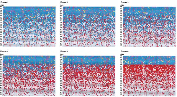
Animation 7.1. Rapid propagation of retirement behavior through social networks, no mandatory retirement age.

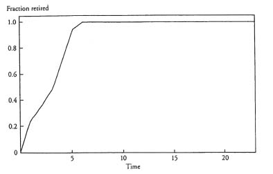
Figure 7.3. Fraction of eligible agents retired over time, typical realization, 15 percent rational agents.

Some Sensitivity Analysis

Each of the realizations described above yields interesting qualitative information about the model. However, in order to characterize the model's overall behavior quantitatively, it is necessary to make many realizations for a particular set of parameters and progressively build up a statistical portrait of the solution space computationally. That is, the intrinsic stochasticity of the model can be approximately characterized through a sufficiently large number of realizations. Once this is done for a particular configuration, one can study the effect of varying parameters. We first define a base case configuration of the model:

Parameter	Value
Agents/cohort (C)	100
Rational agents	10 percent
Imitative agents	85 percent
Imitation threshold (τ)	0.50
Social network size (S)	U[10, 25]
Network age extent (E)	U[0, 5]
Random agents	5 percent
P	0.50

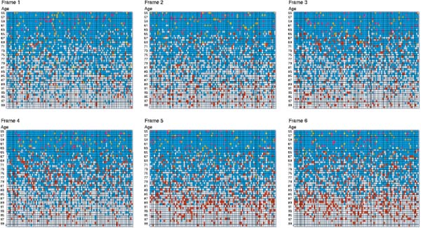
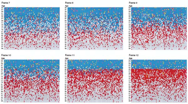
Animation 7.2. Slow propagation of retirement behavior through social networks, no mandatory retirement age.

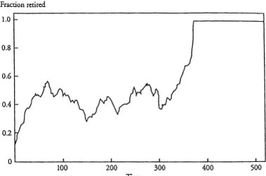
Figure 7.4. Fraction of eligible agents retired over time, typical realization, 5 percent rational agents.

We study the effect of each of these parameters on the time required for the age sixty-five retirement norm to emerge, the transition time. The first parameter, the number of agents per cohort (C), was found to have no effect on the average transition time for C > 100. So we begin our exploration of the model by varying the relative proportions of the three agent types—rationals, imitators, and randoms—keeping all other parameters as in the base case. We performed fifty realizations for each configuration of the model and estimated mean transition times along with standard deviations. Figure 7.5 shows the average transition times for three levels of randomly behaving agents as a function of the fraction of rationals (and hence imitators). Note that the ordinate is in logarithmic coordinates; error bars are ±1 standard deviation and are asymmetrical, due to the logarithmic scale.

Reducing the proportion of rationals, while holding constant the proportion of randoms, increases transition time. When randoms comprise 0 or 5 percent of the population, certain minimum proportions of the population must be rational for a retirement age norm to arise. For a given fraction of rationals, the transition time decreases as the proportion of randoms increases. Notice that the variances increase rapidly with transition times.

Our next sensitivity analysis concerns the effect of the imitation threshold (τ) on transition time. Since social networks are composed of individuals, the fraction of agents in a given network who are engaged in some behavior can only take on certain discrete values. That is, small changes in τ may have no effect on agent decision making, and thus no effect on transition times. For example, imagine that all agents have social networks of size ten. Clearly, increasing τ from 0.55 to 0.58 has no effect; agents either have five or fewer retired agents in their network or they have six or more. Only when τ is moved across a discrete boundary, such as from 0.58 to 0.62, is there an effect.

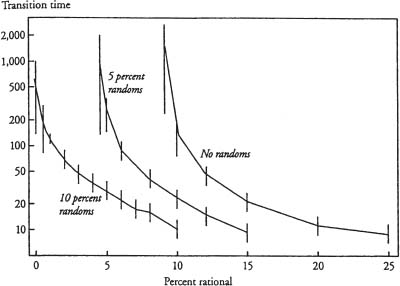
Figure 7.5. Effect of fraction of rational agents on transition to age 65 retirement norm, by fraction of randomly behaving agents.

Therefore instead of studying the dependence of transition times on the average imitation threshold—surely a very “lumpy” dependence—we investigate the effect of making the threshold progressively more heterogeneous in the agent population while holding the average value of τ constant. Figure 7.6 shows how transition times depend on the standard deviation in the imitation threshold, with the average threshold fixed at 0.50. Once again, the ordinate is in logarithmic coordinates. Increasing the variance in the threshold decreases the average transition time. The reason is that in high-variance populations there are relatively more agents with low thresholds, and these agents quickly retire, leading the rest of the population to retire quickly as well. Note that when there is low variance in the imitation threshold, there is significantly more variance in transition time.

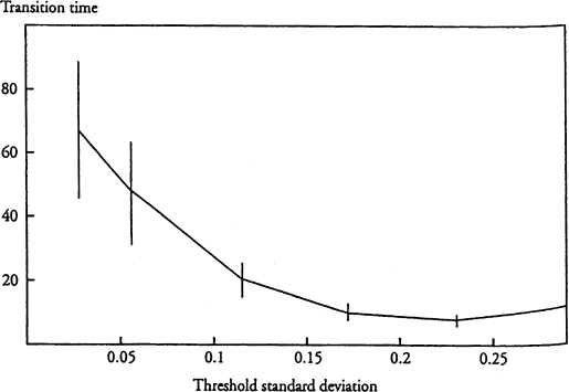
Figure 7.6. Effect of standard deviation in imitation threshold on transition to age 65 retirement norm.

The three panels of figure 7.7 explore the dependence of transition time on the size of agent networks (S). The separate (and opposite) effects of changing the average size and the size variance are presented in the first two panels. They are combined to produce the overall effect shown in the third panel. In particular, the first panel describes the effect of increasing network size, holding variance constant. Note that the time required to transit to a uniform retirement age increases very rapidly with increasing social network size; in large networks, it is difficult for a new norm to become established. The second panel gives the dependence of the transition time on the dispersion (the population standard deviation) in social network size, holding the average size constant. In this case, as the variance increases the transition time decreases, although this is a relatively weak effect. The reason for this is that the small networks catalyze the transition to a new norm, and as the variance increases, there are more small networks.

These two effects are combined in the third panel, where the abscissa, call it represents the maximum size of any social network; that is, the size (S) of an agent's network is set by drawing a random number from U[10,]. As increases, both the average social network size and the variance rise, and the two competing effects on transition time given in the first two panels of the figure play out, yielding the third panel. Overall, the general effect is that the transition time increases very rapidly with .

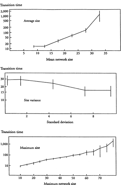
Figure 7.7. Effect of size of social network on transition to age 65 retirement norm.

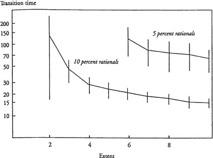
Figure 7.8. Effect of extent of social network on transition to age 65 retirement norm, by fraction of rational agents.

Next, we consider the effect of increasing the extent of agent social networks in the age cohort dimension (E). Throughout the discussion above, the maximum extent of a social network has been five cohorts above and below an agent's own cohort. Figure 7.8 shows the effect of varying this parameter. Note that increasing the extent of agent social networks in the age dimension decreases transition times. The reason for this is that networks having greater extent include older agents, who are more likely to be retired.

Dynamics and “As If”

Notice that in figure 7.6 the only variable affected by the fraction of rationals is the transition time. The attainment, per se, of the age sixty-five retirement norm is compatible with any rationality fraction above a critical level. So while in establishing the social norm, the system does behave “as if” all agents are rational, it also behaves “as if” none are! However, in taking a long time to achieve the norm it does not behave “as if” all agents are rational; indeed, it behaves as if most are not.

RESPONSE TO POLICY CHANGE: SHIFTING THE RETIREMENT AGE FROM SIXTY-FIVE TO SIXTY-TWO

Above, our model permitted agents to retire when they wished; no mandatory retirement age was in effect. We now require that all agents retire at age seventy. This increases the speed at which the age sixty-five retirement norm is established. We wish to investigate the effect of policy interventions on retirement age norms. Therefore once the norm of sixty-five is established, we throw a “policy switch” and lower the retirement age to sixty-two, mimicking the 1961 policy change by Congress. In our model, this switch means only that rationals claim benefits at age sixty-two and that randoms and imitators may receive benefits at age sixty-two. We measure how long it takes for a new retirement age norm to become established. Keep in mind that when the age of eligibility for social security benefits was lowered from sixty-five to sixty-two, it took nearly thirty-five years for a new norm to emerge (see figure 7.1). In animation 7.3, with rationals and randoms each constituting 5 percent of the population, τ distributed on U[0.5, 1.0], and the social networks as in the base case, a new norm emerges after some twenty periods. In short, the model replicates the sluggish adjustment that in fact occurred, at least qualitatively.

We have made many realizations of this model, varying the number of rationals in the population. The results are shown in figure 7.9. Note that the transition time to the age sixty-two norm falls as the fraction of rational agents increases. Based on this parameterization of the model, a new norm is instituted in about thirty-five periods if between 1 and 4 percent of the population responds rationally—that is to say, immediately—to the new policy. The sensitivity analyses described in figures 7.6 through 7.8 indicate how the speed of adjustment depends on other parameters in the model. In particular, we expect the time required to adjust to a policy shock to rise for less variance in the imitation threshold τ and for increases in the average size and extent of social networks.

This use of the agent-based computational model as a kind of laboratory in which alternative policies can be studied seems to us a fertile application of the technology, and one that has not been systematically exploited.

TWO SUBPOPULATIONS, LOOSELY COUPLED BY SOCIAL NETWORKS

Some subgroups in society may be better informed and educated than others. Such differences can affect the relative rates at which these communities adopt various norms. In animation 7.4 the agents have been divided into two distinct subpopulations of the same size: the agents on the left do not include any rational agents, while of the agents on the right, 10 percent are rationals. Other parameters are as in the base case configuration. The two subpopulations are coupled through their social networks as follows: 10 percent of each agent's network belongs to the other subpopulation, with the remainder belonging to its own group. We term this quantity—10 percent—the coupling between subpopulations. Even this rather loose coupling is sufficient for the group containing some rationals to pull the other into conformity with its retirement norm, as shown in animation 7.4.

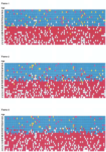
Animation 7.3. Propagation of retirement behavior through social networks, mandatory retirement age of 70 and policy change from earliest retirement age of 65 to 62.

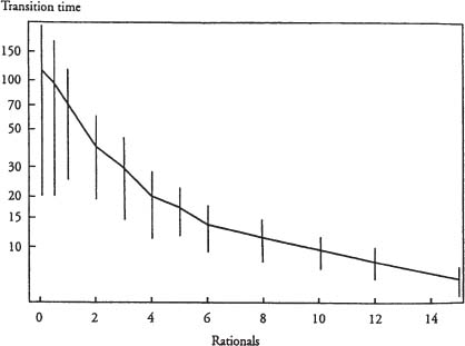
Figure 7.9. Effect of fraction of rational agents on transition to age 62 retirement norm.

We have studied this general effect by systematically varying the extent of coupling between subpopulations and measuring the times required for each group to reach a retirement norm of age sixty-five from an initially unretired state. The results are shown in figure 7.10; each point is an average of over fifty realizations. Note that very little coupling is needed for the nonrational subpopulation to be pulled into conformity with the more rational subpopulation.

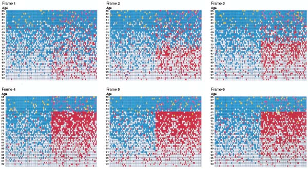
Animation 7.4. Retirement dynamics in two loosely coupled subpopulations.

Figure 7.10. Effect of social network coupling on transition to age 65 retirement norm.

CONCLUSIONS

With social network interactions and imitative dynamics, very little individual rationality may be needed for society as a whole ultimately to exhibit optimal behavior. More pointedly, there is a large literature, experimental and theoretical, devoted to the question: how rational are individual humans? From the perspective of network imitation, it may not matter. Moreover, the nonequilibrium dynamics and the social patchiness of a response to policy will depend on both the size and the structure of networks. It is not clear how one would adapt the representative agent approach to study either of these dependencies. However, they are naturally explored within the agent-based computational framework.

This chapter has barely scratched the surface of a rich and promising area of study. Many fruitful avenues for future research suggest themselves, both analytical and computational. On the analytical side, it would be extremely useful to have—for the transient networks we describe—theorems analogous to those of Lawrence Blume and H. Peyton Young, which give conditions under which social norms will be established eventually for static networks (Blume 1995; Young 1998). Furthermore, it would be desirable to have formal expressions for the way in which transition time distributions depend on model parameters such as the fraction of imitators and size of social networks.

Computationally, it would be useful to extend our model of retirement age norms to include income shocks and imitative consumption behavior over the life cycle, as in the agent-based model of Christopher Carroll and Todd Allen (1997). We suspect that doing so would add more heterogeneity to the outcomes observed in our model. Furthermore, such a model would provide a useful laboratory in which to explore new theoretical ideas, like the effect of hyperbolic discounting, as well as to experiment with policy alternatives, like increasing the retirement age or privatizing social security.

While we have interpreted this model as applying to retirement, it could be applied to a wide range of settings in which social interactions mediate purely rational behavior. Obvious candidates include contagion behavior in markets, migration to different health plans, or the diffusion of technological innovations. In reality, these phenomena occur in social networks, while most existing models treat them either as occurring in “perfectly mixed” environments or via local interactions on regular lattices or other highly specialized topologies. The agent-based computational approach is well suited to studying such processes with any topology of interactions.

APPENDIX A. IMPLEMENTATION OF THE MODEL: AGENTS AS OBJECTS

There are many ways to computationally implement agent-based models. This can be done in any modern programming language, or with any of several mathematical or simulation software packages. However, since the model is stated in terms of individual agents, there is one idea from modern computer science that renders the implementation both transparent and efficacious: object-oriented programming.

Objects are contiguous blocks of memory that contain both data (socalled instance variables) and functions for modifying these data (the object's so-called methods). This ability of objects to hold both data and functions operating on data is called encapsulation.¹⁵ Agent-based models are very naturally implemented using objects, by interpreting an object's data as an agent's state information and the object's functions as the agent's rules of behavior. A population of agents who have the same behavioral repertoire but local state information is then conveniently implemented as multiple instantiations of a single agent object type or class.¹⁶

We have implemented the model described in the text using object-oriented programming. Not only are individual agents objects, but so too are cohorts, albeit objects of a different class than agents. In fact, it has proven convenient for the population of cohorts as a whole to be an object as well.

The agent object has a variety of state variables and behavioral methods. An agent's state information includes type (rational, imitator, or random), age, current employment status (working or retired), and the age at which it will die (“death age”).¹⁷ All of this information is stored locally, in the agent object. Each agent also keeps track of some number of other agents who are identified as its social network. These data are maintained in a social network object, described below. The agent's main decision in the present model is whether or not to retire: this is the agent object's basic method. This agent object specification is summarized as follows:

Pseudo-Code Block 1: Agent Object

OBJECT agent;

   type;

   death_age;

   alive_or_dead;

   social_network;

   working_or_retired;

   next_agent_in_agent_list;

   FUNCTION initialize;

   FUNCTION retirement_decision;

   FUNCTION draw.

In practice, it makes sense to implement as private some of these data and methods—that is, accessible only to the agent to whom they belong—while others are public, although this is not essential.¹⁸

Each social network is also conveniently implemented as an object. The size of each social network is data local to that object, as is an array of pointers to (that is, memory addresses of) the agents who constitute the network. Methods associated with this object include routines for determining how many agents in the network are eligible to retire, and how many are actually retired. This social network object specification is summarized as follows:

Pseudo-Code Block 2: Social Network Object

OBJECT social_network;

   size;

   array_of_agents;

   FUNCTION initialize;

   FUNCTION number_eligible_to_retire;

   FUNCTION number_retired;

   FUNCTION fraction_retired_of_eligible;

   FUNCTION draw.

 

Cohorts are also implemented as objects. The size of the cohort is kept as local data, as is an array of agents who constitute the cohort. The methods of this object are primarily data-gathering and statistical routines, useful in characterizing the behavior of the cohort overall. The cohort object is summarized as follows:

Pseudo-Code Block 3: Cohort Object

OBJECT cohort;

   size;

   array_of_agents;

   FUNCTION initialize;

   FUNCTION average_social_network_size_among_agents_in_cohort;

   FUNCTION number_retired;

   FUNCTION fraction_retired_of_eligible;

   FUNCTION draw.

 

The population of cohorts is also an object. Similar to the cohort object, it is merely an array of entities (here, cohorts), together with data gathering and statistical methods for discerning the state of the population overall.

Putting all of this together, the agent-based computational model amounts to

1. initializing all agents, social networks, and cohorts;
2. choosing an agent at random and incrementing its age;
3. checking to see if the agent has achieved its death age; if yes, then go to 2; else
4. having the agent decide whether to retire;
5. repeat 2 through 4 for all agents;
6. periodically gather and report statistics on the population.

This algorithm is summarized as follows:

Pseudo-Code Block 4: Overall Model

PROGRAM retirement;

initialize agents;

initialize social networks;

initialize cohorts;

repeat:

select an agent at random;

increment its age;

if age < death_age then do

retirement_decision;

get statistics on the agents and cohorts;

until user terminates.

The object model is largely responsible for the relatively compact description of this code.¹⁹

REFERENCES

Axelrod, Robert. 1997. The Complexity of Cooperation. Princeton: Princeton University Press.

Blume, Lawrence. 1995. The Statistical Mechanics of Strategic Interaction. Games and Economic Behavior 5:387-424.

Burtless, Gary. 1986. Social Security, Unanticipated Benefit Increases, and the Timing of Retirement. Review of Economic Studies 53:781-805.

Camerer, Colin. 1997. Progress in Behavioral Game Theory. Journal of Economic Perspectives 11(4): 167-88.

Carroll, Christopher, and Todd Allen. 1997. Learning about Intertemporal Choice. Paper presented at the Santa Fe Institute Workshop on Local Interactions Models in Economics, Santa Fe, NM.

Epstein, Joshua M., and Robert L. Axtell. 1996. Growing Artificial Societies: Social Science from the Bottom Up. Washington, DC: Brookings Institution Press; Cambridge: MIT Press.

Jennings, Nicholas R., Katia Sycara, and Michael Wooldridge. 1998. A Roadmap of Agent Research and Development. Autonomous Agents and Multi-Agent Systems 1(1): 7-38.

Kochen, Manfred, ed. 1989. The Small World. Norwood, NJ: Ablex.

Laibson, David I., Andrea Repetto, and Jeremy Tobacman. 1998. Self-Control and Retirement Savings: Do 401(k)'s Help? Working paper, Harvard University.

Rabin, Matthew. 1998. Psychology and Economics. Journal of Economic Literature 36(1): 11-46.

Rust, John, and Christopher Phelan. 1997. How Social Security and Medicare Affect Retirement Behavior in a World of Incomplete Markets. Econometrica 65(4): 781-831.

Scott, John. 1991. Social Network Analysis. Newbury Park, CA: Sage.

Young, H. Peyton. 1998. Diffusion in Social Networks. Working paper, Brookings Institution.

---

^* Thanks are due George Akerlof, Chris Carroll, Bob Hall, Peyton Young, and participants in the Brookings Work-in-Progress seminar. Research assistance from Trisha Brandon and David Hines is gratefully acknowledged. This research was partially supported by the National Science Foundation, under grant IRI-9725302.

This essay was published previously in Behavioral Dimensions of Retirement Economics, edited by Henry J. Aaron. 1999. Washington, D.C.: Brookings Institution Press; New York: Russell Sage Foundation.

¹ See the recent review in Rabin 1998.

² We thank Gary Burtless for supplying these data.

³ See, for instance, Burtless 1986.

⁴ See, for example, Rust and Phelan 1997; Laibson, Repetto, and Tobacman 1998.

⁵ Certain variables in our model are assigned random values. In all cases below, the random variables are assumed to be uniformly distributed. The uniform (that is, rectangular) distribution on the interval [a, b] is denoted U[a, b].

⁶ The number of cohorts, number of agents per cohort, and distribution of death ages are all easily modified in the software that we have created for this model.

⁷ In the computational implementation of the model, the order of agent activation is randomized within cohorts in each period. It is commonly held that such randomization is necessary in order to suppress so-called simulation artifacts, that is, spurious correlation in the agent population.

⁸ For more on social networks, see Kochen 1989 and Scott 1991

⁹ It makes a difference to the numerical results whether an agent considers all agents in its social network or only those who are eligible to retire. The qualitative character of the results described below, however, does not dependon this distinction.

¹⁰ This development closely follows Young (1998, 3-4).

¹¹ Coordination games on fixed social networks have been studied by Blume (1995) and Young (1998). But because our networks are transient, their analytical results donot apply.

¹² For extended discussions of the agent-based computational approach, see Epstein and Axtell 1996; Axelrod 1997.

¹³ For more on the comparative advantages of this modeling technique, see Epstein and Axtell 1996.

¹⁴ QuickTime™ movies are available on the CD accompanying this book.

¹⁵ Other features of the object model, such as inheritance and polymorphism, seem to be less relevant to agent-based computational models than encapsulation.

¹⁶ For a discussion of the distinction between object and agent, see Jennings, Sycara, and Wooldridge 1998.

¹⁷ The agent is assumed not to know its death age.

¹⁸ Private data and methods are accessible only to the agent to whom they belong, unless other objects are given special access privileges.

¹⁹ The actual source code is less than 2,000 lines of C++ and compiles in the CodeWarrior environment for the Macintosh. A Java implementation is available on the CD accompanying this book.