Prelude to Chapter 12
GENERATING EPIDEMIC DYNAMIC
I LOVE MATHEMATICS. I also believe that mathematical theories can offer fundamental insights. In areas where there is a well-developed and powerful mathematical theory, one should master the theory before building an agent model. Moreover, it is often of great value to “dock” the agent model—or some special case of it—to the classical mathematical one.
In the field of epidemiology, there is a beautiful underlying mathematical theory that applies powerfully to an important class of cases. While we offer an agent-based epidemic model in chapter 12, the effort began with a “docking exercise” worth recounting as a prelude.
The Kermack-McKendrick Equations
Perhaps the most famous equations of mathematical epidemiology are the Kermack-McKendrick equations, published in 1927.1 In the basic model, the total population is constant and is comprised of three homogeneous pools: Susceptibles S(t), Infectives I(t), and Removeds R(t). Conceptually, susceptibles contract the disease through contact with infectives; the infected are then removed from circulation through death or permanent immunity. Since the flow is from susceptible (S) to infective (I) to removed (R), it is termed an SIR epidemic model.2 The flow from state to state is governed by three differential equations. Letting r denote the infection rate (the per contact transmission probability) and p the rate at which infectives are removed from circulation (e.g., by death), the Kermack-McKendrick model is


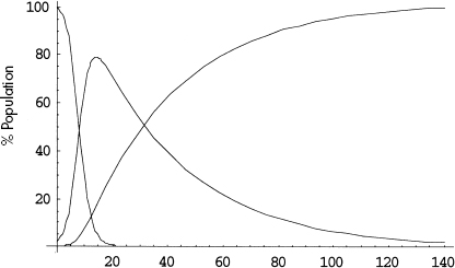
Figure 12.P.1. Illustrative time series solution. Note: S(t) is monotonically decreasing, R(t) monotonically increasing, and I(t) rises and then falls.
A typical solution of this system is graphed in figure 12.P.1.
The susceptible curve falls, as individuals contract the disease and transfer into the infective pool. Accordingly, the infective curve rises. But, after a period of growth, this curve begins to fall also, as agents are removed from circulation, through death or permanent immunity, for example.
Now these equations assume a type of perfect mixing with which we will dispense in the agent-based smallpox model proper. In particular, the equations posit that the rate of flow from the susceptible to the infective pool dS/dt is proportional to the product of the pool sizes, S(t) and I(t). Implicitly, the model lines up all S susceptibles in a row. Then each of the I infectives marches down the entire line of susceptibles and sneezes in each one's face. That produces SI contacts. That's perfect mixing, and the model is very unrealistic in many cases. So what? Realism per se is overrated. It is a very revealing model! Two important and counterintuitive insights are immediate, and they apply even in the agent model we will ultimately build. Indeed, an agent model incapable of capturing them will be of dubious value.
First Counterintuitive Insight: Herd Immunity
Imagine a contagious disease of some sort. And imagine that you possess a perfectly effective vaccine for that disease. Intuition would surely suggest that, to prevent epidemics of the disease, it is necessary to vaccinate the entire population. The Kermack-McKendrick equations say otherwise! How?
To say that an epidemic occurs is to say that the infectious pool, I(t), is growing. In other words, dI/dt > 0. But, by (2), this occurs if and only if rSI > pI, which is to say

The ratio on the right—the removal rate over the infection rate—is a threshold. If the susceptible pool exceeds it, the infection spreads. If not, the epidemic fizzles. The very important implication of this threshold result is that less than universal immunization is required to prevent epidemics. Indeed, by (4), the fraction immunized need only be big enough that the unimmunized fraction—the remaining susceptible pool, S—be below the threshold p/r. Not every cow needs to be immune for the herd to be immune. For instance, diphtheria and scarlet fever require 80 percent immunization to achieve “herd immunity,”3 as the effect is known. Hethcote and Yorke argue that “a vaccine could be very effective in controlling gonorrhea…for a vaccine that gives an average immunity of 6 months, the calculations suggest that random immunization of ½ of the general population each year would cause gonorrhea to disappear.”3 While our smallpox model will differ profoundly from the Kermack-McKendrick picture, the goal of herd immunity is at the core of our vaccination strategy.
Second Counterintuitive Insight
As for the second insight, consider the following proposition: The more deadly a disease is to the individual, the more widespread is the epidemic it produces. Right? Surprisingly, the answer is no, and this, too, is evident from the threshold equation (4). The equation says that if we vaccinate until the remaining susceptible (i.e., unvaccinated) pool falls below p/r, the epidemic will fizzle. So, for the sake of argument, fix r (contagiousness per contact). Now, as p (individual deadliness) gets higher and higher, so does p/r, and we need to vaccinate fewer and fewer to achieve herd immunity. In the limit of perfect deadliness, we don't need to vaccinate anyone: the disease kills off its hosts before they can spread the disease to others, precluding any epidemic! The original proposition is not right. A disease can be so deadly to the individual that it can't spread efficiently. (Smallpox, as we shall see, is more clever than that.)
The Kermack-McKendrick equations, highly idealized as they may be, thus offer two fundamental qualitative insights. And, as a first activity, our team built an extremely simple agent model to “dock” to that classic model.
An Agent Model
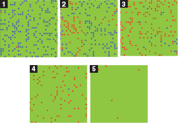
In this minimal agent model, events transpire on a green “playground,” if you like. Healthy susceptible agents are colored blue, while a few initial infective agents are colored red. As an approximation to Kermack-McKendrick perfect mixing, agents move to neighboring sites randomly (they execute a 2D random walk in their von Neumann neighborhoods), bumping into other agents. Any time an infective (red) bumps into a healthy (blue), the disease is transmitted with fixed probability (0.2), just as in Kermack-McKendrick. And, as in that model, there is no heterogeneity within the susceptible or infective pools, and infectives are removed (die) with probability 0.4 per period. A movie of the typical epidemic is on the CD. Snapshots are offered in run 1.
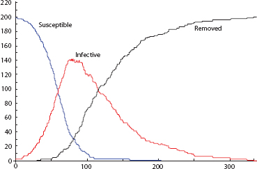
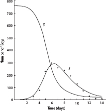
Over time, the blue population turns red, as susceptibles contract the disease, and reds disappear, as they are removed from circulation. The time series are exactly as in the figure 12.P.1 solution curves for the Kermack-McKendrick model, as shown in figure 12.P.2. So this is a reasonable “docking” of an agent model to the classic one. Moreover, they both do very nicely in cases where the well-mixed assumption holds, as in the data from a 1978 influenza epidemic in an English boys’ school shown in figure 12.P.3. The epidemic took place in winter on a small campus where dining commons and dormitories ensured high contact rates, permitting the well-mixed model to apply nicely. Notice the close fit between theoretical and observed infective curves.

Run 1. Agent Kermack-McKendrick model.

Figure 12.P.2. Agent time series.

Figure 12.P.3. Influenza epidemic data, 1978, English boarding school. Of 763 boys, 512 were confined to bed, 22 January-February 1978. (Source: British Medical Journal, 4 March 1978.)
For modeling the spread of smallpox in modern urban settings, however, this well-mixed assumption can be dangerously misleading, and we will depart from it. Some degree of spatial realism is fundamentally important. Agents, moreover, will need to be heterogeneous in a variety of important ways not reflected in the Kermack-McKendrick model.
However, that model, and explicit mathematical models in general, are very important tools. We are all prisoners of our tools. But if one must live in a prison cell, one would like it to be as spacious as possible. So one should try to master all the tools one can.
1 W. O. Kermack and A. G. McKendrick, “Contributions to the Mathematical Theory of Epidemics,” Proceedings of the Royal Statistical Society, ser. A, 115:700-721.
2 For a thorough modern mathematical exposition, see Paul Waltman, Deterministic Threshold Models in the Theory of Epidemics (New York: Springer, 1974).
3 Leah Edelstein-Keshet, Mathematical Models in Biology (New York: Random House, 1988), 255.
4 H. W. Hethcote and J. A. Yorke, Gonorrhea Transmission Dynamics and Control (New York: Springer, 1980).