APPENDIX
Research Design
This book makes two key claims, which are summarized in the introduction as follows:
Claim A. For states in the global South with substantial levels of public debt, a high export concentration in point-source natural resources (particularly fuels and minerals), imported in large and growing quantities by China, was a necessary but not sufficient condition for a break with neoliberal policy orientation during the years 2002 to 2013.
Claim B. For each resource-exporting state, whether such a break occurred—as well as its form and direction—depended primarily upon the dynamics of its domestic state–society relations.
Qualitative comparative analysis is used to test claim A, and the results are summarized in chapter 3. This appendix provides a more detailed rundown of the research design pertaining to this aspect of the book. The use of Charles Ragin’s (1989, 2008) qualitative comparative analysis approach means that some of the common methodological trade-offs in deciding between qualitative and comparative may be transcended, to some extent. Briefly, QCA mimics the thickness of qualitative case-based comparative studies but enables the comparison of a much larger number of cases than is typically possible with such methods. It does so by following case-based analysis with the reduction of each case to a configuration of conditions (the equivalent of variables in QCA nomenclature), which then may be easily compared.
I employ QCA in the first stage of this research in order to assess the credibility of the central hypothesis and to explore for other potentially causally important conditions, using a set of nineteen cases from the global South. Even though many of the conditions I set out here are based in quantitative indicators, it is still the case that their selection and operationalization are both theoretically informed and rely on an understanding of individual cases and their contexts.
QCA was also chosen because it is particularly suitable for testing causality in terms of necessary conditions, even if it is perhaps most commonly associated with for tests of sufficiency (see, for example, Rihoux et al. 2013; Kirchherr, Charles, and Walton 2016). The use of QCA as a first stage in a mixed-methods approach is well established (Liebermann 2005; Schneider and Rohlfing 2013). However, in much of the discussion on mixed methods, the goal is to combine two methods to generate and/or test the same hypothesis (or hypotheses), with, for example, a small number of case studies being used to establish a series of claims, which are then tested across a method like QCA, which allows for greater generalizability.
The research design here is different because the two methods used (QCA for claim A and case studies/typology formation for claim B) focus on testing and elaborating two different (but linked) hypotheses. The second stage, typology formation (the subject of chapters 4 through 9), involves a process of detailed case-based investigation, followed by the drawing out of sometimes quite complex dynamics and processes within the cases, and then finally an abstraction of these features into distinct types. QCA’s basis in an operation of reducing cases to a series of discrete values indicating the presence or absence of fixed conditions means that it was not suitable for the second stage of research (though, with the typology now in hand, one potential way to extend the book’s findings would be to test the claims that inform the typology, using QCA on a larger set of cases). Theoretical and methodological concerns relating to typology formation (and claim B) were dealt with in chapter 4. The rest of this appendix, therefore, is devoted to the QCA stage and the testing of claim A.
Making an empirical claim about the presence of one variable enabling, but not causing, a change in the value of another variable requires a different formulation than the probabilistic relationship assumed in most statistical models. QCA allows for this by considering outcomes and causes as subsets of one another. Cast in set-theoretic terms, my hypothesis may be restated as “instances of Southern states breaking with neoliberalism are a subset of instances of Southern states with high export concentrations in hard commodities demanded by China.” Here, the outcome (break with neoliberalism) is presented as a subset of the cause (states with high export concentrations in resources). Expressed another way, the cause is a necessary but not sufficient condition for the occurrence of the outcome.
I define a break with neoliberalization as the adoption of an overall policy trajectory on the part of a given government that would not have been acceptable to international financial institutions or donors during the neoliberal era of the 1980s and 1990s and thus would have been impossible to enact without a highly damaging rupture with creditors or Development Assistance Committee members. Importantly, I conceptualize this as a question of direction of travel (i.e., whether a state’s policies are oriented toward continuing neoliberalization or along a different trajectory), rather than of starting and ending points. So, for example, Venezuela is usually understood as having undergone less extensive neoliberal reform over the 1980s and 1990s than, say, Bolivia (Lora 2012), but nevertheless as having neoliberalized to some extent. I see Venezuela as having made a break with neoliberalism during the commodity boom period not because it was, so to speak, less neoliberalized than other cases at the end of the boom but because it shifted from an overall orientation of liberalization to a substantially different policy direction over the period (see chapter 6).
Since QCA demands relatively in-depth research on all cases used in the analysis, some initial selection to narrow down the number of cases to be considered is required, for reasons of practicality. The solution adopted here, in line with recommended practice within QCA (Rihoux and Lobe 2009), is to reduce the number of cases to a manageable level by identifying and selecting cases based on theoretically relevant background conditions. Though this may at times result in somewhat arbitrary cutoffs, a benefit is that such a method effectively controls for these conditions and therefore simplifies the identification of causality within each case. These scoping conditions do limit the applicability of the findings, in the first instance at least, to those cases considered. However, since the QCA (as well as the later empirical chapters) are concerned with the specification of causal mechanisms rather than simply correlation of cause and effect, the results, while not strictly generalizable outside the limits of the scoping conditions, should at least suggest whether similar mechanisms might apply, and in which cases.
First, all cases are drawn from the global South. The boundaries of the global South are somewhat subject to interpretation, but for the purposes of this analysis, I take it to include all states in Africa, Asia, Latin America, and the Pacific with a per capita gross domestic product lower than $20,000 in 2002 (World Bank n.d.).
Second, levels of indebtedness seem to have an important role to play both in neoliberalization and in putative breaks with it. High levels of public debt imply a lack of fiscal space with which to engage in discretionary spending, as well as a likely reliance upon IFI loans or aid, bringing the imposition of policy stipulations. A condition relating to debt levels thus does two things. First, it sets a higher bar for the hypothesis, in that the fiscal impact of China-driven export revenues (whether direct or indirect) must be significant enough to negate this strong prior debt constraint. Southern states with low levels of debt may find it much easier, should they wish, to adopt non-neoliberal policies without any help from hard commodity export revenues, given the weaker disciplinary strength of IFIs and financial markets that this implies. Second, all things being equal, highly indebted Southern states, through the extended reach of market discipline into their political economies, are likely to have experienced higher levels of neoliberalization than their less indebted counterparts. I therefore limit the case selection to states with external debt stocks equivalent to 40 percent or more of gross national income at the beginning of the commodity boom, using the average figure for 2001 and 2002 in order to smooth out any large temporary swings that may have occurred over these years (World Bank n.d.).
As a third scoping condition, it is assumed that any identifiable move away from neoliberalization requires a minimal level of political stability in order to successfully implement a chosen policy direction. For this reason, I rule out any states that experienced wars, revolutions, or sustained periods of widespread civil and political turmoil over the years 2002 to 2013.
Fourth, I exclude small states with populations under 10 million (as of 2016) (World Bank n.d.), which may be may be more easily influenced by external forces (Haggard and Kaufman 1989). Controlling for such conditions, even imperfectly, again enhances the comparability of cases. Further, a few states are omitted from consideration, owing to a lack of data on one or more of the conditions analyzed in the next section of this appendix. This leaves eighteen states from across the global South (including sub-Saharan Africa, Latin America, East Asia, and Central Asia) as cases for QCA analysis (see table A.1).
Change in liberalization, 2001/2002–2013/2014
|
Angola |
−0.64 |
Ghana |
+0.54 |
Philippines |
0.96 |
||||
|
Argentina |
−1.37 |
Indonesia |
+0.49 |
Senegal |
+0.60 |
||||
|
Bolivia |
−0.34 |
Kazakhstan |
−0.51 |
Tanzania |
+1.24 |
||||
|
Brazil |
−0.48 |
Malawi |
+0.43 |
Uganda |
+0.84 |
||||
|
Ecuador |
−1.13 |
Malaysia |
+0.95 |
Venezuela |
−0.41 |
||||
|
Ethiopia |
+0.19 |
Peru |
+0.30 |
Zambia |
+0.06 |
Source: Calculated from Fraser Institute, Economic Freedom dataset.
Analysis of Necessary Conditions
This section lists the conditions employed, for testing as to their possible necessity, and gives the theoretical rationale for their selection as potentially causally significant. Since I use the crisp set version of QCA, all conditions have only two possible (Boolean) values: 1, indicating the presence of the condition, or 0, indicating its absence. I explain how data has been operationalized and values of 1 or 0 have been specified in relation to each condition. Conditions are constructed by comparing the beginning of the boom with its end. The 2008–2009 crisis fell in the middle of this period and obviously had a major impact upon commodity markets, prompting interest in the ability of some resource exporters to use countercyclical policies in ways that had not been available to them during previous crises (Griffith-Jones and Ocampo 2009). I briefly discussed some of these moves in relation to particular cases in the book’s later chapters. However, since this episode turned out to be a temporary pause rather than the end of the boom, here I look at changes that occurred over the whole length of the period.
• BRK: This is the outcome condition. A value of 1 indicates that the given state made a break with neoliberalism over the course of the commodity boom, whereas a value of 0 indicates that it did not. There have been several attempts over the years to put together inexes of liberalization across developing world economies. However, these tend to be limited in geographic coverage or in the indicators they survey (Lora 2012; Morley, Machado, and Pettinato 1999; Sachs and Warner 1995; Wacziarg and Welch 2008). Others seek to measure more expansive sets of indicators, such as institutional quality along with liberalization (as in the World Bank’s Country Policy and Institutional Assessment scores). Two right-wing think tanks, the Heritage Foundation and the Fraser Institute, publish annual rankings of what they refer to as “economic freedom.” On the face of it, neither of these is especially useful, because both conflate data on policy changes (such as rates of taxation or tariffs) with economic outcomes (such as the rate of inflation), as well as with broader issues beyond the realm of economic policy choice (as in the Fraser Institute giving a score for the impartiality of a country’s court system). Naturally, putting these rather different categories together results in a ranking that tends to show those states with well-functioning institutions and good economic performance as the most economically free—precisely because all of these things are taken as indicators of economic freedom—lending a tautological character to these judgments.
However, the Fraser Institute’s (n.d.) Economic Freedom dataset, in particular, is a useful source of data for my purposes. By selecting only indicators relating to core areas of economic liberalization, I construct an index that is used as the basis for scoring cases on the BRK condition. These indicators are size of government (based on share of government consumption in the economy, transfers and subsidies, state-owned enterprises and state investment, and top marginal tax rates); trade (tariff rates and nontariff barriers); and labor market regulations. Each of these three areas is scored from 0 (least liberalized) to 10 (most liberalized), on an annualized basis. I calculate overall scores for each case from a simple average across my three indicators.
Table A.2 shows the change in score between the average for 2001/2002 and the average for 2013/2014, for all eighteen cases. Positive scores indicate an overall increase in liberalization over the period and are assigned a 0 value on the BRK condition. Negative scores indicate a decrease in liberalization and thus are assigned a 1 value on the BRK condition (that is, as breaks with liberalization). Data for Angola, Ethiopia, and Kazakhstan only extends back to 2005, so for these cases, the change in liberalization shown in the table is calculated from the difference between the 2005 score and the 2013/2014 average.
Qualitative comparative analysis truth table
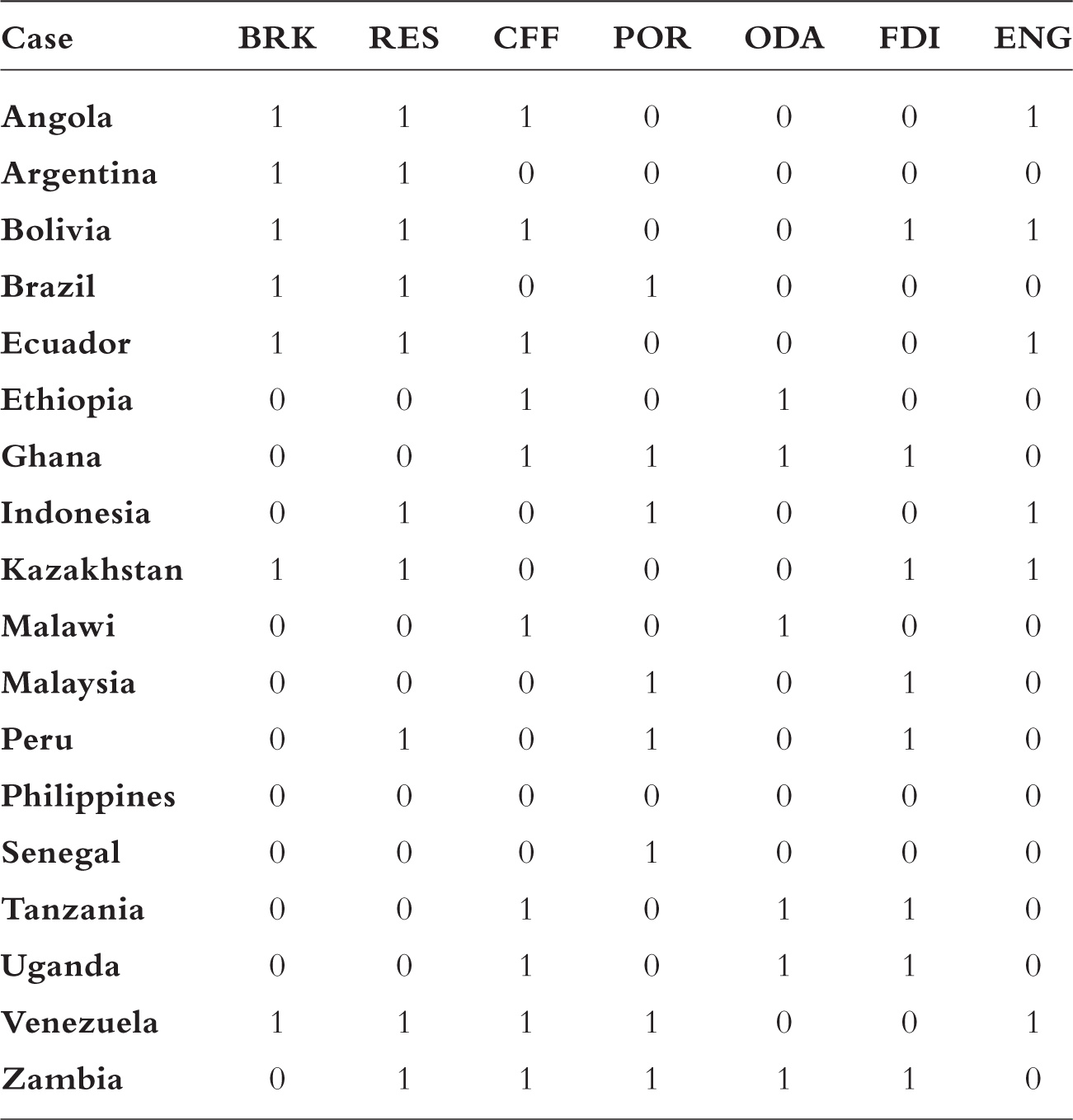
• RES: This is the hypothesized necessary condition, indicating the absence or presence of a substantial export sector in energy commodities (crude petroleum, natural gas, and coking/metallurgical coal) and metals (including ores and refined metals, excluding gold and silver, and not including alloys or manufactures) subject to the China effect on prices and demand. As was explained in detail in chapter 5, this total also includes soybeans (and minimally processed soy products), because China’s demand impact on the market for soybeans is comparable to that in metals and minerals, and because the particular structure of the soybean industry means that it has certain similarities with extractive sectors, uniquely among agricultural products that make up a substantial share of exports in any of the cases examined.
A score of 1 on this condition indicates a case for which total exports of commodities of this type averaged 25 percent or more of total merchandise exports during the 2002–2013 period. Data is drawn from the Chatham House Resourcetrade Database (Chatham House n.d.) and the UNCTADStat data center (United Nations Conference on Trade and Development n.d.). Alternative operationalizations are possible, using resource exports as a percentage of GDP or of government revenue. I deem the government revenue measure unsuitable because this partially depends upon government policy such as taxation and royalty levels, which themselves make up part of the outcome value (as a potential part of policy moves toward and away from a neoliberal trajectory). The 25 percent of exports threshold is adopted as being in line with conventions in much of the relevant academic and policy literature (see, for instance, Haglund 2011; Thomas et al. 2011) and on the basis of readily available data over the full period.
• ENG: Similar to the RES condition, but counting toward the 25 percent threshold export concentration exclusively in fuels (oil, natural gas, and coal) and excluding other natural resource commodities such as metals. This condition is included as a means of distinguishing between the causal impacts of natural resource export sectors in general and fossil fuels specifically. Data is again taken from the Chatham House Resourcetrade database.
• FDI: It is plausible that high levels of foreign direct investment may limit states’ range of policy choices, in the sense that a market-friendly orientation may be required (or perceived to be required) on the part of a government to attract or sustain inward investment. Membership of this set covers those states whose average annual inward FDI flows as a percentage of GDP over the 2002–2013 period exceed the developing country average of 2.7 percent (calculated from UNCTADStat data center). This measure was adopted in preference to an indicator based on FDI stocks because FDI stocks may reflect legacies of investment undertaken before the period studied and therefore may have occurred under different global conditions (considering that extractive capital, in particular, tends to be relatively immobile). Also considered was inward FDI as a proportion of gross capital formation, though this was rejected on the grounds that gross capital formation appears to be correlated, to some degree, with level of development.
• ODA: The set of cases classified as being dependent on official development assistance, in the sense that the degree of reliance upon foreign aid to finance basic state functions means that donors control budgetary resources to an extent that may impose significant constraints on states’ abilities to set policy independently. A standard measure of aid intensity is total aid flows per annum as a percentage of GDP, with a suggested threshold of 10 percent for aid-dependent status (Brautigam and Knack 2004). World Bank World Development Indicators give the slightly different but equivalent measure of net official development assistance (including concessional loans) as a percentage of gross national income. I use a threshold of 10 percent or more on this metric, averaged across 2002, for a case to score 1 on this condition. I reviewed the notion of aid dependence in chapter 8.
• CFF: Chinese financial flows. Tracking Chinese overseas finance is somewhat complicated by a lack of transparency in officially released numbers and by the fact that these flows do not always fit neatly into standard categories as per, for example, Organisation for Economic Co-operation and Development definitions of concessional finance (Brautigam 2011). This condition is meant to capture the totality of official Chinese financial flows, including aid (which is a relatively small component) as well as other official financing streams directed to governments and SOEs in each of the cases. In this sense, it is meant to represent a way to test for the causal impact of Chinese development finance, as analogous to the role of IFIs and established donors. The extent to which Chinese flows might differ in character, and the implications for recipient states in terms of policy autonomy, is a subject that has garnered considerable interest in the literature (Woods 2008; Gallagher, Irwin, and Koleski 2012; McEwan and Mawdsley 2012; Kragelund 2015).
I draw on AidData’s Global Chinese Official Finance Dataset (Dreher et al. 2017) here, which covers the period 2000 to 2014. Earlier versions of this dataset have attracted some criticism (Brautigam 2013) for its reliance on media reports for data collection. However, newer versions appear to have addressed many of the earlier concerns. While the authors readily admit that this is a second-best source in the absence of reliable official data, it is nevertheless the only dataset of its type that spans all geographic regions of the South. I take note of the authors’ advice by including only records marked “Recommended for research,” these being projects at either the commitment, implementation, or completion stage (rather than those that have only been pledged). I score membership of this set based on total Chinese financial flows received as a percentage of 2014 GDP (International Monetary Fund n.d.), with a threshold of 4 percent. I come to this figure based on an appraisal of the significance of Chinese official finance in the various cases. Venezuela appears to have the lowest total (at 4.5 percent) among states where such financing has, on the face of it, played a major in the political-economic course of the period (Muchapondwa et al. 2016).
• POR: This condition measures changes in net portfolio investment in the balance of payments account for each case over the years 2002 to 2013. This is meant to give an indication of the behavior of external investors, in light of the possibility that their withdrawal of capital might serve to “punish” moves on the part of states to shift away from orthodoxy liberal policies (Campello 2007; compare with Block 1977). Here, I score cases as belonging to this set when they have an average annual net outflow of 0.5 percent of GDP or higher. Though movements in portfolio investment are likely to be affected by factors other than markets’ judgments on policy choices, this nevertheless sets up a test of whether breaks from neoliberalism can take place in conditions of sustained capital flight over the period. What this condition does not test for is the impact of sudden capital stops.
Table A.2 gives the data used for the QCA in tabulated format (known as a truth table), showing the scores for each case across the range of conditions. Performing an analysis of necessary conditions for the outcome BRK (Using fsQCA software) gives the results shown in table A.3.
Table A.3 lists results of testing the presence or absence of each condition as a possible necessary condition for the outcome (BRK). The presence of a tilde (~) before a condition indicates a set negation—that is, testing for the absence of that condition. Consistency scores give a measure of the degree to which cases with a positive score on the outcome value are a subset of cases with a positive score for each particular condition. For instance, the consistency score of 1 for the condition RES, as shown in the table, means that cases where the outcome is present (that is, where a break with neoliberalism took place) are a subset of those where the condition RES is present (that is, those cases that are resource exporters). Thus, all cases where a break with neoliberalism took place are resource exporters—making the latter a necessary condition for the former. Significantly, ~ODA (that is, an absence of official development assistance dependence) is also a necessary condition for a break with neoliberalism to take place. I discussed this finding in more detail in the case study chapters, particularly chapter 8.
Analysis of necessary conditions
|
Condition tested |
Consistency |
Coverage |
||
|
RES |
1.000000 |
0.636364 |
||
|
ENG |
0.714286 |
0.833333 |
||
|
CFF |
0.571429 |
0.363636 |
||
|
POR |
0.285714 |
0.222222 |
||
|
ODA |
0.000000 |
0.000000 |
||
|
FDI |
0.285714 |
0.222222 |
||
|
~RES |
0.000000 |
0.000000 |
||
|
~CFF |
0.428571 |
0.375000 |
||
|
~POR |
0.714286 |
0.500000 |
||
|
~ODA |
1.000000 |
0.538462 |
||
|
~FDI |
0.714286 |
0.500000 |
||
|
~ENG |
0.285714 |
0.153846 |
Outcome variable: BRK
Some caution needs to be exercised here, particularly given the scoping conditions used to select cases (such as levels of indebtedness or population size), which limits the generalizability of the results, to some degree. Nevertheless, this finding is strong evidence in favor of my claim that a high concentration in resource exports demanded by China is indeed a necessary condition for a break with neoliberalism on the part of Southern states.
Coverage scores also are provided for each condition. These show the extent to which instances of a condition are a subset of those in which the outcome is present—essentially, the degree to which they are sufficient conditions for breaks with neoliberalism to take place. As can be seen, none of the conditions tested were alone sufficient for the outcome. However, ENG, the condition denoting a high export concentration in energy commodities, has a high coverage score—in fact, of the cases where ENG is present, only Indonesia did not break with neoliberalism.
The ten cases belonging to the set RES in the analysis make up the bulk of the cases explored in the typology chapters (chapters 4 through 9). I increase the set of typology cases to fifteen by relaxing the conditions on debt and population, in order to include Jamaica, Laos, Mongolia, South Africa, and Colombia in the comparison.
Interviews
Three of the cases included in the typology (Ecuador, Zambia, and Jamaica) are partly informed by short periods of fieldwork in each location over the course of 2013. Anonymous interviews are cited in relation to these cases in chapters 6, 8, and 9, corresponding to the lists of interviewees in tables A.4, A.5, and A.6.
Ecuador interviews
|
Interview Number |
Organization |
Position |
||
|
1e |
Universidad Andina Simón Bolívar |
Academic |
||
|
2e |
Universidad San Francisco de Quito |
Academic |
||
|
3e |
Opposition party |
Politician |
||
|
4e |
Private Banking Association |
Official |
||
|
5e |
West European Embassy |
Official |
||
|
6e |
— |
Former finance minister |
||
|
7e |
Patriotic Society Party |
Politician |
||
|
8e |
Chamber of Commerce, Guayaquil |
Official |
||
|
9e |
Chamber of Industry and Production, Quito |
Official |
||
|
10e |
NGO (environment) |
Official |
||
|
11e |
National Secretariat of Planning and Development (SENPLADES) |
Official |
Zambia interviews
|
Interview Number |
Organization |
Position |
||
|
1z |
Transnational mining firm |
Official |
||
|
2z |
Norwegian embassy |
Official |
||
|
3z |
British embassy |
Official |
||
|
4z |
International financial institution |
Official |
||
|
5z |
— |
Former opposition party politician |
||
|
6z |
German Development Agency |
Official |
||
|
7z |
University of Zambia |
Academic |
||
|
8z |
United Party for National Development |
Politician |
||
|
9z |
Patriotic Front |
Local organizer |
Jamaica interviews
|
Interview Number |
Organization |
Position |
||
|
1j |
University of West Indies |
Academic |
||
|
2j |
Jamaica Labour Party |
Former minister |
||
|
3j |
People’s National Party |
Politician |
||
|
4j |
Mining company |
Bauxite mining expert |
||
|
5j |
Planning Institute of Jamaica |
Official |
||
|
6j |
Nongovernmental organization |
Official |
||
|
7j |
Private Sector Organisation of Jamaica |
Official |
||
|
8j |
Jamaica Chamber of Commerce |
Official |
||
|
9j |
— |
Former senator |