Vector Processors in More Depth
Revised by Krste Asanovic, Massachusetts Institute of Technology
I’m certainly not inventing vector processors. There are three kinds that I know of existing today. They are represented by the Illiac-IV, the (CDC) Star processor, and the TI (ASC) processor. Those three were all pioneering processors.…One of the problems of being a pioneer is you always make mistakes and I never, never want to be a pioneer. It’s always best to come second when you can look at the mistakes the pioneers made.
Seymour Cray Public lecture at Lawrence Livermore Laboratorieson on the introduction of the Cray-1 (1976)
G.1 Introduction
Chapter 4 introduces vector architectures and places Multimedia SIMD extensions and GPUs in proper context to vector architectures.
In this appendix, we go into more detail on vector architectures, including more accurate performance models and descriptions of previous vector architectures. Figure G.1 shows the characteristics of some typical vector processors, including the size and count of the registers, the number and types of functional units, the number of load-store units, and the number of lanes.

If the machine is a multiprocessor, the entries correspond to the characteristics of one processor. Several of the machines have different clock rates in the vector and scalar units; the clock rates shown are for the vector units. The Fujitsu machines’ vector registers are configurable: The size and count of the 8K 64-bit entries may be varied inversely to one another (e.g., on the VP200, from eight registers each 1K elements long to 256 registers each 32 elements long). The NEC machines have eight foreground vector registers connected to the arithmetic units plus 32 to 64 background vector registers connected between the memory system and the foreground vector registers. Add pipelines perform add and subtract. The multiply/divide-add unit on the Hitachi S810/820 performs an FP multiply or divide followed by an add or subtract (while the multiply-add unit performs a multiply followed by an add or subtract). Note that most processors use the vector FP multiply and divide units for vector integer multiply and divide, and several of the processors use the same units for FP scalar and FP vector operations. Each vector load-store unit represents the ability to do an independent, overlapped transfer to or from the vector registers. The number of lanes is the number of parallel pipelines in each of the functional units as described in Section G.4. For example, the NEC SX/5 can complete 16 multiplies per cycle in the multiply functional unit. Several machines can split a 64-bit lane into two 32-bit lanes to increase performance for applications that require only reduced precision. The Cray SV1 and Cray X1 can group four CPUs with two lanes each to act in unison as a single larger CPU with eight lanes, which Cray calls a Multi-Streaming Processor (MSP).
G.2 Vector Performance in More Depth
The chime approximation is reasonably accurate for long vectors. Another source of overhead is far more significant than the issue limitation.
The most important source of overhead ignored by the chime model is vector start-up time. The start-up time comes from the pipelining latency of the vector operation and is principally determined by how deep the pipeline is for the functional unit used. The start-up time increases the effective time to execute a convoy to more than one chime. Because of our assumption that convoys do not overlap in time, the start-up time delays the execution of subsequent convoys. Of course, the instructions in successive convoys either have structural conflicts for some functional unit or are data dependent, so the assumption of no overlap is reasonable. The actual time to complete a convoy is determined by the sum of the vector length and the start-up time. If vector lengths were infinite, this start-up overhead would be amortized, but finite vector lengths expose it, as the following example shows.
Example
Assume that the start-up overhead for functional units is shown in Figure G.2.

Show the time that each convoy can begin and the total number of cycles needed. How does the time compare to the chime approximation for a vector of length 64?
Answer
Figure G.3 provides the answer in convoys, assuming that the vector length is n. One tricky question is when we assume the vector sequence is done; this determines whether the start-up time of the SV is visible or not. We assume that the instructions following cannot fit in the same convoy, and we have already assumed that convoys do not overlap. Thus, the total time is given by the time until the last vector instruction in the last convoy completes. This is an approximation, and the start-up time of the last vector instruction may be seen in some sequences and not in others. For simplicity, we always include it.

The vector length is n.
The time per result for a vector of length 64 is 4 + (42/64) = 4.65 clock cycles, while the chime approximation would be 4. The execution time with startup overhead is 1.16 times higher.
For simplicity, we will use the chime approximation for running time, incorporating start-up time effects only when we want performance that is more detailed or to illustrate the benefits of some enhancement. For long vectors, a typical situation, the overhead effect is not that large. Later in the appendix, we will explore ways to reduce start-up overhead.
Start-up time for an instruction comes from the pipeline depth for the functional unit implementing that instruction. If the initiation rate is to be kept at 1 clock cycle per result, then

For example, if an operation takes 10 clock cycles, it must be pipelined 10 deep to achieve an initiation rate of one per clock cycle. Pipeline depth, then, is determined by the complexity of the operation and the clock cycle time of the processor. The pipeline depths of functional units vary widely—2 to 20 stages are common—although the most heavily used units have pipeline depths of 4 to 8 clock cycles.
For VMIPS, we will use the same pipeline depths as the Cray-1, although latencies in more modern processors have tended to increase, especially for loads. All functional units are fully pipelined. From Chapter 4, pipeline depths are 6 clock cycles for floating-point add and 7 clock cycles for floating-point multiply. On VMIPS, as on most vector processors, independent vector operations using different functional units can issue in the same convoy.
In addition to the start-up overhead, we need to account for the overhead of executing the strip-mined loop. This strip-mining overhead, which arises from

These are the start-up penalties in clock cycles for VMIPS vector operations.
the need to reinitiate the vector sequence and set the Vector Length Register (VLR) effectively adds to the vector start-up time, assuming that a convoy does not overlap with other instructions. If that overhead for a convoy is 10 cycles, then the effective overhead per 64 elements increases by 10 cycles, or 0.15 cycles per element.
Two key factors contribute to the running time of a strip-mined loop consisting of a sequence of convoys:
- 1. The number of convoys in the loop, which determines the number of chimes. We use the notation Tchime for the execution time in chimes.
- 2. The overhead for each strip-mined sequence of convoys. This overhead consists of the cost of executing the scalar code for strip-mining each block, Tloop, plus the vector start-up cost for each convoy, Tstart.
There may also be a fixed overhead associated with setting up the vector sequence the first time. In recent vector processors, this overhead has become quite small, so we ignore it.
The components can be used to state the total running time for a vector sequence operating on a vector of length n, which we will call Tn:

The values of Tstart, Tloop, and Tchime are compiler and processor dependent. The register allocation and scheduling of the instructions affect both what goes in a convoy and the start-up overhead of each convoy.
For simplicity, we will use a constant value for Tloop on VMIPS. Based on a variety of measurements of Cray-1 vector execution, the value chosen is 15 for Tloop. At first glance, you might think that this value is too small. The overhead in each loop requires setting up the vector starting addresses and the strides, incrementing counters, and executing a loop branch. In practice, these scalar instructions can be totally or partially overlapped with the vector instructions, minimizing the time spent on these overhead functions. The value of Tloop of course depends on the loop structure, but the dependence is slight compared with the connection between the vector code and the values of Tchime and Tstart.
Example
What is the execution time on VMIPS for the vector operation A = B × s, where s is a scalar and the length of the vectors A and B is 200?
Answer
Assume that the addresses of A and B are initially in Ra and Rb, s is in Fs, and recall that for MIPS (and VMIPS) R0 always holds 0. Since (200 mod 64) = 8, the first iteration of the strip-mined loop will execute for a vector length of 8 elements, and the following iterations will execute for a vector length of 64 elements. The starting byte addresses of the next segment of each vector is eight times the vector length. Since the vector length is either 8 or 64, we increment the address registers by 8 × 8 = 64 after the first segment and 8 × 64 = 512 for later segments. The total number of bytes in the vector is 8 × 200 = 1600, and we test for completion by comparing the address of the next vector segment to the initial address plus 1600. Here is the actual code:
      DADDUI   R2,R0,#1600 ;total # bytes in vector
      DADDU    R2,R2,Ra    ;address of the end of A vector
      DADDUI   R1,R0,#8    ;loads length of 1st segment
      MTC1     VLR,R1      ;load vector length in VLR
      DADDUI   R1,R0,#64   ;length in bytes of 1st segment
      DADDUI   R3,R0,#64   ;vector length of other segments
Loop: LV       V1,Rb       ;load B
      MULVS.D  V2,V1,Fs    ;vector * scalar
      SV       Ra,V2       ;store A
      DADDU    Ra,Ra,R1    ;address of next segment of A
      DADDU    Rb,Rb,R1    ;address of next segment of B
      DADDUI   R1,R0,#512  ;load byte offset next segment
      MTC1     VLR,R3      ;set length to 64 elements
      DSUBU    R4,R2,Ra    ;at the end of A?
      BNEZ     R4,Loop     ;if not, go back
The three vector instructions in the loop are dependent and must go into three convoys, hence Tchime = 3. Let’s use our basic formula:

The value of Tstart is the sum of:
Thus, the value of Tstart is given by:

So, the overall value becomes:

The execution time per element with all start-up costs is then 784/200 = 3.9, compared with a chime approximation of three. In Section G.4, we will be more ambitious—allowing overlapping of separate convoys.
Figure G.5 shows the overhead and effective rates per element for the previous example (A = B × s) with various vector lengths. A chime-counting model would lead to 3 clock cycles per element, while the two sources of overhead add 0.9 clock cycles per element in the limit.

For short vectors, the total start-up time is more than one-half of the total time, while for long vectors it reduces to about one-third of the total time. The sudden jumps occur when the vector length crosses a multiple of 64, forcing another iteration of the strip-mining code and execution of a set of vector instructions. These operations increase Tn by Tloop + Tstart.
Pipelined Instruction Start-Up and Multiple Lanes
Adding multiple lanes increases peak performance but does not change start-up latency, and so it becomes critical to reduce start-up overhead by allowing the start of one vector instruction to be overlapped with the completion of preceding vector instructions. The simplest case to consider is when two vector instructions access a different set of vector registers. For example, in the code sequence
ADDV.D V1,V2,V3
ADDV.D V4,V5,V6
An implementation can allow the first element of the second vector instruction to follow immediately the last element of the first vector instruction down the FP adder pipeline. To reduce the complexity of control logic, some vector machines require some recovery time or dead time in between two vector instructions dispatched to the same vector unit. Figure G.6 is a pipeline diagram that shows both start-up latency and dead time for a single vector pipeline.

Each element has a 5-cycle latency: 1 cycle to read the vector-register file, 3 cycles in execution, then 1 cycle to write the vector-register file. Elements from the same vector instruction can follow each other down the pipeline, but this machine inserts 4 cycles of dead time between two different vector instructions. The dead time can be eliminated with more complex control logic. (Reproduced with permission from Asanovic [1998].)
The following example illustrates the impact of this dead time on achievable vector performance.
Pipelining instruction start-up becomes more complicated when multiple instructions can be reading and writing the same vector register and when some instructions may stall unpredictably—for example, a vector load encountering memory bank conflicts. However, as both the number of lanes and pipeline latencies increase, it becomes increasingly important to allow fully pipelined instruction start-up.
G.3 Vector Memory Systems in More Depth
To maintain an initiation rate of one word fetched or stored per clock, the memory system must be capable of producing or accepting this much data. As we saw in Chapter 4, this usually done by spreading accesses across multiple independent memory banks. Having significant numbers of banks is useful for dealing with vector loads or stores that access rows or columns of data.
The desired access rate and the bank access time determined how many banks were needed to access memory without stalls. This example shows how these timings work out in a vector processor.
Example
Suppose we want to fetch a vector of 64 elements starting at byte address 136, and a memory access takes 6 clocks. How many memory banks must we have to support one fetch per clock cycle? With what addresses are the banks accessed? When will the various elements arrive at the CPU?
Answer
Six clocks per access require at least 6 banks, but because we want the number of banks to be a power of 2, we choose to have 8 banks. Figure G.7 shows the timing for the first few sets of accesses for an 8-bank system with a 6-clock-cycle access latency.

Each memory bank latches the element address at the start of an access and is then busy for 6 clock cycles before returning a value to the CPU. Note that the CPU cannot keep all 8 banks busy all the time because it is limited to supplying one new address and receiving one data item each cycle.
The timing of real memory banks is usually split into two different components, the access latency and the bank cycle time (or bank busy time). The access latency is the time from when the address arrives at the bank until the bank returns a data value, while the busy time is the time the bank is occupied with one request. The access latency adds to the start-up cost of fetching a vector from memory (the total memory latency also includes time to traverse the pipelined interconnection networks that transfer addresses and data between the CPU and memory banks). The bank busy time governs the effective bandwidth of a memory system because a processor cannot issue a second request to the same bank until the bank busy time has elapsed.
For simple unpipelined SRAM banks as used in the previous examples, the access latency and busy time are approximately the same. For a pipelined SRAM bank, however, the access latency is larger than the busy time because each element access only occupies one stage in the memory bank pipeline. For a DRAM bank, the access latency is usually shorter than the busy time because a DRAM needs extra time to restore the read value after the destructive read operation. For memory systems that support multiple simultaneous vector accesses or allow nonsequential accesses in vector loads or stores, the number of memory banks should be larger than the minimum; otherwise, memory bank conflicts will exist.
Memory bank conflicts will not occur within a single vector memory instruction if the stride and number of banks are relatively prime with respect to each other and there are enough banks to avoid conflicts in the unit stride case. When there are no bank conflicts, multiword and unit strides run at the same rates. Increasing the number of memory banks to a number greater than the minimum to prevent stalls with a stride of length 1 will decrease the stall frequency for some other strides. For example, with 64 banks, a stride of 32 will stall on every other access, rather than every access. If we originally had a stride of 8 and 16 banks, every other access would stall; with 64 banks, a stride of 8 will stall on every eighth access. If we have multiple memory pipelines and/or multiple processors sharing the same memory system, we will also need more banks to prevent conflicts. Even machines with a single memory pipeline can experience memory bank conflicts on unit stride accesses between the last few elements of one instruction and the first few elements of the next instruction, and increasing the number of banks will reduce the probability of these inter-instruction conflicts. In 2011, most vector supercomputers spread the accesses from each CPU across hundreds of memory banks. Because bank conflicts can still occur in non-unit stride cases, programmers favor unit stride accesses whenever possible.
A modern supercomputer may have dozens of CPUs, each with multiple memory pipelines connected to thousands of memory banks. It would be impractical to provide a dedicated path between each memory pipeline and each memory bank, so, typically, a multistage switching network is used to connect memory pipelines to memory banks. Congestion can arise in this switching network as different vector accesses contend for the same circuit paths, causing additional stalls in the memory system.
G.4 Enhancing Vector Performance
In this section, we present techniques for improving the performance of a vector processor in more depth than we did in Chapter 4.
Chaining in More Depth
Early implementations of chaining worked like forwarding, but this restricted the timing of the source and destination instructions in the chain. Recent implementations use flexible chaining, which allows a vector instruction to chain to essentially any other active vector instruction, assuming that no structural hazard is generated. Flexible chaining requires simultaneous access to the same vector register by different vector instructions, which can be implemented either by adding more read and write ports or by organizing the vector-register file storage into interleaved banks in a similar way to the memory system. We assume this type of chaining throughout the rest of this appendix.
Even though a pair of operations depends on one another, chaining allows the operations to proceed in parallel on separate elements of the vector. This permits the operations to be scheduled in the same convoy and reduces the number of chimes required. For the previous sequence, a sustained rate (ignoring start-up) of two floating-point operations per clock cycle, or one chime, can be achieved, even though the operations are dependent! The total running time for the above sequence becomes:

Figure G.8 shows the timing of a chained and an unchained version of the above pair of vector instructions with a vector length of 64. This convoy requires one chime; however, because it uses chaining, the start-up overhead will be seen in the actual timing of the convoy. In Figure G.8, the total time for chained operation is 77 clock cycles, or 1.2 cycles per result. With 128 floating-point operations done in that time, 1.7 FLOPS per clock cycle are obtained. For the unchained version, there are 141 clock cycles, or 0.9 FLOPS per clock cycle.

The 6- and 7-clock-cycle delays are the latency of the adder and multiplier.
Although chaining allows us to reduce the chime component of the execution time by putting two dependent instructions in the same convoy, it does not eliminate the start-up overhead. If we want an accurate running time estimate, we must count the start-up time both within and across convoys. With chaining, the number of chimes for a sequence is determined by the number of different vector functional units available in the processor and the number required by the application. In particular, no convoy can contain a structural hazard. This means, for example, that a sequence containing two vector memory instructions must take at least two convoys, and hence two chimes, on a processor like VMIPS with only one vector load-store unit.
Chaining is so important that every modern vector processor supports flexible chaining.
Sparse Matrices in More Depth
Chapter 4 shows techniques to allow programs with sparse matrices to execute in vector mode. Let’s start with a quick review. In a sparse matrix, the elements of a vector are usually stored in some compacted form and then accessed indirectly. Assuming a simplified sparse structure, we might see code that looks like this:
          do       100 i = 1,n
100                A(K(i)) = A(K(i)) + C(M(i))
This code implements a sparse vector sum on the arrays A and C, using index vectors K and M to designate the nonzero elements of A and C. (A and C must have the same number of nonzero elements—n of them.) Another common representation for sparse matrices uses a bit vector to show which elements exist and a dense vector for the nonzero elements. Often both representations exist in the same program. Sparse matrices are found in many codes, and there are many ways to implement them, depending on the data structure used in the program.
A simple vectorizing compiler could not automatically vectorize the source code above because the compiler would not know that the elements of K are distinct values and thus that no dependences exist. Instead, a programmer directive would tell the compiler that it could run the loop in vector mode.
More sophisticated vectorizing compilers can vectorize the loop automatically without programmer annotations by inserting run time checks for data dependences. These run time checks are implemented with a vectorized software version of the advanced load address table (ALAT) hardware described in Appendix H for the Itanium processor. The associative ALAT hardware is replaced with a software hash table that detects if two element accesses within the same stripmine iteration are to the same address. If no dependences are detected, the stripmine iteration can complete using the maximum vector length. If a dependence is detected, the vector length is reset to a smaller value that avoids all dependency violations, leaving the remaining elements to be handled on the next iteration of the strip-mined loop. Although this scheme adds considerable software overhead to the loop, the overhead is mostly vectorized for the common case where there are no dependences; as a result, the loop still runs considerably faster than scalar code (although much slower than if a programmer directive was provided).
A scatter-gather capability is included on many of the recent supercomputers. These operations often run more slowly than strided accesses because they are more complex to implement and are more susceptible to bank conflicts, but they are still much faster than the alternative, which may be a scalar loop. If the sparsity properties of a matrix change, a new index vector must be computed. Many processors provide support for computing the index vector quickly. The CVI (create vector index) instruction in VMIPS creates an index vector given a stride (m), where the values in the index vector are 0, m, 2 × m, …, 63 × m. Some processors provide an instruction to create a compressed index vector whose entries correspond to the positions with a one in the mask register. Other vector architectures provide a method to compress a vector. In VMIPS, we define the CVI instruction to always create a compressed index vector using the vector mask. When the vector mask is all ones, a standard index vector will be created.
The indexed loads-stores and the CVI instruction provide an alternative method to support conditional vector execution. Let us first recall code from Chapter 4:
     low = 1
     VL = (n mod MVL) /*find the odd-size piece*/
     do 1 j = 0,(n/MVL) /*outer loop*/
         do 10 i = low, low + VL - 1 /*runs for length VL*/
              Y(i) = a * X(i) + Y(i) /*main operation*/
10        continue
         low = low + VL /*start of next vector*/
         VL = MVL /*reset the length to max*/
1   continue
Here is a vector sequence that implements that loop using CVI:
LV        V1,Ra        ;load vector A into V1
L.D       F0,#0        ;load FP zero into F0
SNEVS.D   V1,F0        ;sets the VM to 1 if V1(i)!=F0
CVI       V2,#8        ;generates indices in V2
POP       R1,VM        ;find the number of 1’s in VM
MTC1      VLR,R1       ;load vector-length register
CVM                    ;clears the mask
LVI       V3,(Ra+V2)    ;load the nonzero A elements
LVI       V4,(Rb+V2)    ;load corresponding B elements
SUBV.D    V3,V3,V4      ;do the subtract
SVI       (Ra+V2),V3    ;store A back
Whether the implementation using scatter-gather is better than the conditionally executed version depends on the frequency with which the condition holds and the cost of the operations. Ignoring chaining, the running time of the original version is 5n + c1. The running time of the second version, using indexed loads and stores with a running time of one element per clock, is 4n + 4fn + c2, where f is the fraction of elements for which the condition is true (i.e., A(i) ¦ 0). If we assume that the values of c1 and c2 are comparable, or that they are much smaller than n, we can find when this second technique is better.

We want Time1 > Time2, so

That is, the second method is faster if less than one-quarter of the elements are nonzero. In many cases, the frequency of execution is much lower. If the index vector can be reused, or if the number of vector statements within the if statement grows, the advantage of the scatter-gather approach will increase sharply.
G.5 Effectiveness of Compiler Vectorization
Two factors affect the success with which a program can be run in vector mode. The first factor is the structure of the program itself: Do the loops have true data dependences, or can they be restructured so as not to have such dependences? This factor is influenced by the algorithms chosen and, to some extent, by how they are coded. The second factor is the capability of the compiler. While no compiler can vectorize a loop where no parallelism among the loop iterations exists, there is tremendous variation in the ability of compilers to determine whether a loop can be vectorized. The techniques used to vectorize programs are the same as those discussed in Chapter 3 for uncovering ILP; here, we simply review how well these techniques work.
There is tremendous variation in how well different compilers do in vectorizing programs. As a summary of the state of vectorizing compilers, consider the data in Figure G.9, which shows the extent of vectorization for different processors using a test suite of 100 handwritten FORTRAN kernels. The kernels were designed to test vectorization capability and can all be vectorized by hand; we will see several examples of these loops in the exercises.

For each processor we indicate how many loops were completely vectorized, partially vectorized, and unvectorized. These loops were collected by Callahan, Dongarra, and Levine [1988]. Two different compilers for the Cray X-MP show the large dependence on compiler technology.
G.6 Putting It All Together: Performance of Vector Processors
In this section, we look at performance measures for vector processors and what they tell us about the processors. To determine the performance of a processor on a vector problem we must look at the start-up cost and the sustained rate. The simplest and best way to report the performance of a vector processor on a loop is to give the execution time of the vector loop. For vector loops, people often give the MFLOPS (millions of floating-point operations per second) rating rather than execution time. We use the notation Rn for the MFLOPS rating on a vector of length n. Using the measurements Tn (time) or Rn (rate) is equivalent if the number of FLOPS is agreed upon. In any event, either measurement should include the overhead.
In this section, we examine the performance of VMIPS on a DAXPY loop (see Chapter 4) by looking at performance from different viewpoints. We will continue to compute the execution time of a vector loop using the equation developed in Section G.2. At the same time, we will look at different ways to measure performance using the computed time. The constant values for Tloop used in this section introduce some small amount of error, which will be ignored.
Measures of Vector Performance
Because vector length is so important in establishing the performance of a processor, length-related measures are often applied in addition to time and MFLOPS. These length-related measures tend to vary dramatically across different processors and are interesting to compare. (Remember, though, that time is always the measure of interest when comparing the relative speed of two processors.) Three of the most important length-related measures are
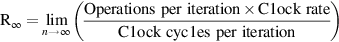
 R∞—The MFLOPS rate on an infinite-length vector. Although this measure may be of interest when estimating peak performance, real problems have limited vector lengths, and the overhead penalties encountered in real problems will be larger.
- N1/2—The vector length needed to reach one-half of R∞. This is a good measure of the impact of overhead.
- Nv—The vector length needed to make vector mode faster than scalar mode. This measures both overhead and the speed of scalars relative to vectors.
Let’s look at these measures for our DAXPY problem running on VMIPS. When chained, the inner loop of the DAXPY code in convoys looks like Figure G.10 (assuming that Rx and Ry hold starting addresses).

Recall our performance equation for the execution time of a vector loop with n elements, Tn:
Chaining allows the loop to run in three chimes (and no less, since there is one memory pipeline); thus, Tchime = 3. If Tchime were a complete indication of performance, the loop would run at an MFLOPS rate of 2/3 × clock rate (since there are 2 FLOPS per iteration). Thus, based only on the chime count, a 500 MHz VMIPS would run this loop at 333 MFLOPS assuming no strip-mining or start-up overhead. There are several ways to improve the performance: Add additional vector load-store units, allow convoys to overlap to reduce the impact of start-up overheads, and decrease the number of loads required by vector-register allocation. We will examine the first two extensions in this section. The last optimization is actually used for the Cray-1, VMIPS’s cousin, to boost the performance by 50%. Reducing the number of loads requires an interprocedural optimization; we examine this transformation in Exercise G.6. Before we examine the first two extensions, let’s see what the real performance, including overhead, is.
The Peak Performance of VMIPS on DAXPY
First, we should determine what the peak performance, R∞, really is, since we know it must differ from the ideal 333 MFLOPS rate. For now, we continue to use the simplifying assumption that a convoy cannot start until all the instructions in an earlier convoy have completed; later we will remove this restriction. Using this simplification, the start-up overhead for the vector sequence is simply the sum of the start-up times of the instructions:

Using MVL = 64, Tloop = 15, Tstart = 49, and Tchime = 3 in the performance equation, and assuming that n is not an exact multiple of 64, the time for an n-element operation is

The sustained rate is actually over 4 clock cycles per iteration, rather than the theoretical rate of 3 chimes, which ignores overhead. The major part of the difference is the cost of the start-up overhead for each block of 64 elements (49 cycles versus 15 for the loop overhead).
We can now compute R∞ for a 500 MHz clock as:
The numerator is independent of n, hence

The performance without the start-up overhead, which is the peak performance given the vector functional unit structure, is now 1.33 times higher. In actuality, the gap between peak and sustained performance for this benchmark is even larger!
Sustained Performance of VMIPS on the Linpack Benchmark
The Linpack benchmark is a Gaussian elimination on a 100 × 100 matrix. Thus, the vector element lengths range from 99 down to 1. A vector of length k is used k times. Thus, the average vector length is given by:
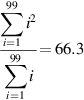
Now we can obtain an accurate estimate of the performance of DAXPY using a vector length of 66:

The peak number, ignoring start-up overhead, is 1.64 times higher than this estimate of sustained performance on the real vector lengths. In actual practice, the Linpack benchmark contains a nontrivial fraction of code that cannot be vectorized. Although this code accounts for less than 20% of the time before vectorization, it runs at less than one-tenth of the performance when counted as FLOPS. Thus, Amdahl’s law tells us that the overall performance will be significantly lower than the performance estimated from analyzing the inner loop.
Since vector length has a significant impact on performance, the N1/2 and Nv measures are often used in comparing vector machines.
Example
What is N1/2 for just the inner loop of DAXPY for VMIPS with a 500 MHz clock?
Answer
Using R∞ as the peak rate, we want to know the vector length that will achieve about 125 MFLOPS. We start with the formula for MFLOPS assuming that the measurement is made for N1/2 elements:
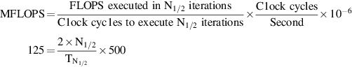
Simplifying this and then assuming N1/2 < 64, so that  , yields:

So N1/2 = 13; that is, a vector of length 13 gives approximately one-half the peak performance for the DAXPY loop on VMIPS.
Example
What is the vector length, Nv, such that the vector operation runs faster than the scalar?
Answer
Again, we know that Nv < 64. The time to do one iteration in scalar mode can be estimated as 10 + 12 + 12 + 7 + 6 + 12 = 59 clocks, where 10 is the estimate of the loop overhead, known to be somewhat less than the strip-mining loop overhead. In the last problem, we showed that this vector loop runs in vector mode in time Tn ≤ 64 = 64 + 3 × n clock cycles. Therefore,
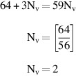
For the DAXPY loop, vector mode is faster than scalar as long as the vector has at least two elements. This number is surprisingly small.
DAXPY Performance on an Enhanced VMIPS
DAXPY, like many vector problems, is memory limited. Consequently, performance could be improved by adding more memory access pipelines. This is the major architectural difference between the Cray X-MP (and later processors) and the Cray-1. The Cray X-MP has three memory pipelines, compared with the Cray-1’s single memory pipeline, and the X-MP has more flexible chaining. How does this affect performance?
Example
What would be the value of T66 for DAXPY on VMIPS if we added two more memory pipelines?
Answer
With three memory pipelines, all the instructions fit in one convoy and take one chime. The start-up overheads are the same, so

With three memory pipelines, we have reduced the clock cycle count for sustained performance from 326 to 194, a factor of 1.7. Note the effect of Amdahl’s law: We improved the theoretical peak rate as measured by the number of chimes by a factor of 3, but only achieved an overall improvement of a factor of 1.7 in sustained performance.
Another improvement could come from allowing different convoys to overlap and also allowing the scalar loop overhead to overlap with the vector instructions. This requires that one vector operation be allowed to begin using a functional unit before another operation has completed, which complicates the instruction issue logic. Allowing this overlap eliminates the separate start-up overhead for every convoy except the first and hides the loop overhead as well.
To achieve the maximum hiding of strip-mining overhead, we need to be able to overlap strip-mined instances of the loop, allowing two instances of a convoy as well as possibly two instances of the scalar code to be in execution simultaneously. This requires the same techniques we looked at in Chapter 3 to avoid WAR hazards, although because no overlapped read and write of a single vector element is possible, copying can be avoided. This technique, called tailgating, was used in the Cray-2. Alternatively, we could unroll the outer loop to create several instances of the vector sequence using different register sets (assuming sufficient registers), just as we did in Chapter 3. By allowing maximum overlap of the convoys and the scalar loop overhead, the start-up and loop overheads will only be seen once per vector sequence, independent of the number of convoys and the instructions in each convoy. In this way, a processor with vector registers can have both low start-up overhead for short vectors and high peak performance for very long vectors.
Example
What would be the values of R∞ and T66 for DAXPY on VMIPS if we added two more memory pipelines and allowed the strip-mining and start-up overheads to be fully overlapped?
Answer

Since the overhead is only seen once, Tn = n + 49 + 15 = n + 64. Thus,

Adding the extra memory pipelines and more flexible issue logic yields an improvement in peak performance of a factor of 4. However, T66 = 130, so for shorter vectors the sustained performance improvement is about 326/130 = 2.5 times.
In summary, we have examined several measures of vector performance. Theoretical peak performance can be calculated based purely on the value of Tchime as:
By including the loop overhead, we can calculate values for peak performance for an infinite-length vector (R∞) and also for sustained performance, Rn for a vector of length n, which is computed as:

Using these measures we also can find N1/2 and Nv, which give us another way of looking at the start-up overhead for vectors and the ratio of vector to scalar speed. A wide variety of measures of performance of vector processors is useful in understanding the range of performance that applications may see on a vector processor.
G.7 A Modern Vector Supercomputer: The Cray X1
The Cray X1 was introduced in 2002, and, together with the NEC SX/8, represents the state of the art in modern vector supercomputers. The X1 system architecture supports thousands of powerful vector processors sharing a single global memory.
The Cray X1 has an unusual processor architecture, shown in Figure G.11. A large Multi-Streaming Processor (MSP) is formed by ganging together four Single-Streaming Processors (SSPs). Each SSP is a complete single-chip vector microprocessor, containing a scalar unit, scalar caches, and a two-lane vector unit. The SSP scalar unit is a dual-issue out-of-order superscalar processor with a 16 KB instruction cache and a 16 KB scalar write-through data cache, both two-way set associative with 32-byte cache lines. The SSP vector unit contains a vector register file, three vector arithmetic units, and one vector load-store unit. It is much easier to pipeline deeply a vector functional unit than a superscalar issue mechanism, so the X1 vector unit runs at twice the clock rate (800 MHz) of the scalar unit (400 MHz). Each lane can perform a 64-bit floating-point add and a 64-bit floating-point multiply each cycle, leading to a peak performance of 12.8 GFLOPS per MSP.

All previous Cray machines could trace their instruction set architecture (ISA) lineage back to the original Cray-1 design from 1976, with 8 primary registers each for addresses, scalar data, and vector data. For the X1, the ISA was redesigned from scratch to incorporate lessons learned over the last 30 years of compiler and microarchitecture research. The X1 ISA includes 64 64-bit scalar address registers and 64 64-bit scalar data registers, with 32 vector data registers (64 bits per element) and 8 vector mask registers (1 bit per element). The large increase in the number of registers allows the compiler to map more program variables into registers to reduce memory traffic and also allows better static scheduling of code to improve run time overlap of instruction execution. Earlier Crays had a compact variable-length instruction set, but the X1 ISA has fixedlength instructions to simplify superscalar fetch and decode.
Four SSP chips are packaged on a multichip module together with four cache chips implementing an external 2 MB cache (Ecache) shared by all the SSPs. The Ecache is two-way set associative with 32-byte lines and a write-back policy. The Ecache can be used to cache vectors, reducing memory traffic for codes that exhibit temporal locality. The ISA also provides vector load and store instruction variants that do not allocate in cache to avoid polluting the Ecache with data that is known to have low locality. The Ecache has sufficient bandwidth to supply one 64-bit word per lane per 800 MHz clock cycle, or over 50 GB/sec per MSP.
At the next level of the X1 packaging hierarchy, shown in Figure G.12, four MSPs are placed on a single printed circuit board together with 16 memory controller chips and DRAM to form an X1 node. Each memory controller chip has eight separate Rambus DRAM channels, where each channel provides 1.6 GB/sec of memory bandwidth. Across all 128 memory channels, the node has over 200 GB/sec of main memory bandwidth.

An X1 system can contain up to 1024 nodes (4096 MSPs or 16,384 SSPs), connected via a very high-bandwidth global network. The network connections are made via the memory controller chips, and all memory in the system is directly accessible from any processor using load and store instructions. This provides much faster global communication than the message-passing protocols used in cluster-based systems. Maintaining cache coherence across such a large number of high-bandwidth shared-memory nodes would be challenging. The approach taken in the X1 is to restrict each Ecache to cache data only from the local node DRAM. The memory controllers implement a directory scheme to maintain coherency between the four Ecaches on a node. Accesses from remote nodes will obtain the most recent version of a location, and remote stores will invalidate local Ecaches before updating memory, but the remote node cannot cache these local locations.
Vector loads and stores are particularly useful in the presence of long-latency cache misses and global communications, as relatively simple vector hardware can generate and track a large number of in-flight memory requests. Contemporary superscalar microprocessors support only 8 to 16 outstanding cache misses, whereas each MSP processor can have up to 2048 outstanding memory requests (512 per SSP). To compensate, superscalar microprocessors have been moving to larger cache line sizes (128 bytes and above) to bring in more data with each cache miss, but this leads to significant wasted bandwidth on non-unit stride accesses over large datasets. The X1 design uses short 32-byte lines throughout to reduce bandwidth waste and instead relies on supporting many independent cache misses to sustain memory bandwidth. This latency tolerance together with the huge memory bandwidth for non-unit strides explains why vector machines can provide large speedups over superscalar microprocessors for certain codes.
Multi-Streaming Processors
The Multi-Streaming concept was first introduced by Cray in the SV1, but has been considerably enhanced in the X1. The four SSPs within an MSP share Ecache, and there is hardware support for barrier synchronization across the four SSPs within an MSP. Each X1 SSP has a two-lane vector unit with 32 vector registers each holding 64 elements. The compiler has several choices as to how to use the SSPs within an MSP.
The simplest use is to gang together four two-lane SSPs to emulate a single eight-lane vector processor. The X1 provides efficient barrier synchronization primitives between SSPs on a node, and the compiler is responsible for generating the MSP code. For example, for a vectorizable inner loop over 1000 elements, the compiler will allocate iterations 0–249 to SSP0, iterations 250–499 to SSP1, iterations 500–749 to SSP2, and iterations 750–999 to SSP3. Each SSP can process its loop iterations independently but must synchronize back with the other SSPs before moving to the next loop nest.
If inner loops do not have many iterations, the eight-lane MSP will have low efficiency, as each SSP will have only a few elements to process and execution time will be dominated by start-up time and synchronization overheads. Another way to use an MSP is for the compiler to parallelize across an outer loop, giving each SSP a different inner loop to process. For example, the following nested loops scale the upper triangle of a matrix by a constant:
/* Scale upper triangle by constant K. */
for (row = 0; row < MAX_ROWS; row++)
  for (col = row; col < MAX_COLS; col++)
     A[row][col] = A[row][col] * K;
Consider the case where MAX_ROWS and MAX_COLS are both 100 elements. The vector length of the inner loop steps down from 100 to 1 over the iterations of the outer loop. Even for the first inner loop, the loop length would be much less than the maximum vector length (256) of an eight-lane MSP, and the code would therefore be inefficient. Alternatively, the compiler can assign entire inner loops to a single SSP. For example, SSP0 might process rows 0, 4, 8, and so on, while SSP1 processes rows 1, 5, 9, and so on. Each SSP now sees a longer vector. In effect, this approach parallelizes the scalar overhead and makes use of the individual scalar units within each SSP.
Most application code uses MSPs, but it is also possible to compile code to use all the SSPs as individual processors where there is limited vector parallelism but significant thread-level parallelism.
Cray X1E
In 2004, Cray announced an upgrade to the original Cray X1 design. The X1E uses newer fabrication technology that allows two SSPs to be placed on a single chip, making the X1E the first multicore vector microprocessor. Each physical node now contains eight MSPs, but these are organized as two logical nodes of four MSPs each to retain the same programming model as the X1. In addition, the clock rates were raised from 400 MHz scalar and 800 MHz vector to 565 MHz scalar and 1130 MHz vector, giving an improved peak performance of 18 GFLOPS.
G.8 Concluding Remarks
During the 1980s and 1990s, rapid performance increases in pipelined scalar processors led to a dramatic closing of the gap between traditional vector supercomputers and fast, pipelined, superscalar VLSI microprocessors. In 2011, it is possible to buy a laptop computer for under $1000 that has a higher CPU clock rate than any available vector supercomputer, even those costing tens of millions of dollars. Although the vector supercomputers have lower clock rates, they support greater parallelism using multiple lanes (up to 16 in the Japanese designs) versus the limited multiple issue of the superscalar microprocessors. Nevertheless, the peak floating-point performance of the low-cost microprocessors is within a factor of two of the leading vector supercomputer CPUs. Of course, high clock rates and high peak performance do not necessarily translate into sustained application performance. Main memory bandwidth is the key distinguishing feature between vector supercomputers and superscalar microprocessor systems.
Providing this large non-unit stride memory bandwidth is one of the major expenses in a vector supercomputer, and traditionally SRAM was used as main memory to reduce the number of memory banks needed and to reduce vector start-up penalties. While SRAM has an access time several times lower than that of DRAM, it costs roughly 10 times as much per bit! To reduce main memory costs and to allow larger capacities, all modern vector supercomputers now use DRAM for main memory, taking advantage of new higher-bandwidth DRAM interfaces such as synchronous DRAM.
This adoption of DRAM for main memory (pioneered by Seymour Cray in the Cray-2) is one example of how vector supercomputers have adapted commodity technology to improve their price-performance. Another example is that vector supercomputers are now including vector data caches. Caches are not effective for all vector codes, however, so these vector caches are designed to allow high main memory bandwidth even in the presence of many cache misses. For example, the Cray X1 MSP can have 2048 outstanding memory loads; for microprocessors, 8 to 16 outstanding cache misses per CPU are more typical maximum numbers.
Another example is the demise of bipolar ECL or gallium arsenide as technologies of choice for supercomputer CPU logic. Because of the huge investment in CMOS technology made possible by the success of the desktop computer, CMOS now offers competitive transistor performance with much greater transistor density and much reduced power dissipation compared with these more exotic technologies. As a result, all leading vector supercomputers are now built with the same CMOS technology as superscalar microprocessors. The primary reason why vector supercomputers have lower clock rates than commodity microprocessors is that they are developed using standard cell ASIC techniques rather than full custom circuit design to reduce the engineering design cost. While a microprocessor design may sell tens of millions of copies and can amortize the design cost over this large number of units, a vector supercomputer is considered a success if over a hundred units are sold!
Conversely, via superscalar microprocessor designs have begun to absorb some of the techniques made popular in earlier vector computer systems, such as with the Multimedia SIMD extensions. As we showed in Chapter 4, the investment in hardware for SIMD performance is increasing rapidly, perhaps even more than for multiprocessors. If the even wider SIMD units of GPUs become well integrated with the scalar cores, including scatter-gather support, we may well conclude that vector architectures have won the architecture wars!
G.9 Historical Perspective and References
This historical perspective adds some details and references that were left out of the version in Chapter 4.
The CDC STAR processor and its descendant, the CYBER 205, were memory-memory vector processors. To keep the hardware simple and support the high bandwidth requirements (up to three memory references per floating-point operation), these processors did not efficiently handle non-unit stride. While most loops have unit stride, a non-unit stride loop had poor performance on these processors because memory-to-memory data movements were required to gather together (and scatter back) the nonadjacent vector elements; these operations used special scatter-gather instructions. In addition, there was special support for sparse vectors that used a bit vector to represent the zeros and nonzeros and a dense vector of nonzero values. These more complex vector operations were slow because of the long memory latency, and it was often faster to use scalar mode for sparse or non-unit stride operations. Schneck [1987] described several of the early pipelined processors (e.g., Stretch) through the first vector processors, including the 205 and Cray-1. Dongarra [1986] did another good survey, focusing on more recent processors.
The 1980s also saw the arrival of smaller-scale vector processors, called mini-supercomputers. Priced at roughly one-tenth the cost of a supercomputer ($0.5 to $1 million versus $5 to $10 million), these processors caught on quickly. Although many companies joined the market, the two companies that were most successful were Convex and Alliant. Convex started with the uniprocessor C-1 vector processor and then offered a series of small multiprocessors, ending with the C-4 announced in 1994. The keys to the success of Convex over this period were their emphasis on Cray software capability, the effectiveness of their compiler (see Figure G.9), and the quality of their UNIX OS implementation. The C-4 was the last vector machine Convex sold; they switched to making large-scale multiprocessors using Hewlett-Packard RISC microprocessors and were bought by HP in 1995. Alliant [1987] concentrated more on the multiprocessor aspects; they built an eight-processor computer, with each processor offering vector capability. Alliant ceased operation in the early 1990s.
In the early 1980s, CDC spun out a group, called ETA, to build a new supercomputer, the ETA-10, capable of 10 GFLOPS. The ETA processor was delivered in the late 1980s (see Fazio [1987]) and used low-temperature CMOS in a configuration with up to 10 processors. Each processor retained the memory-memory architecture based on the CYBER 205. Although the ETA-10 achieved enormous peak performance, its scalar speed was not comparable. In 1989, CDC, the first supercomputer vendor, closed ETA and left the supercomputer design business.
In 1986, IBM introduced the System/370 vector architecture (see Moore et al. [1987]) and its first implementation in the 3090 Vector Facility. The architecture extended the System/370 architecture with 171 vector instructions. The 3090/VF was integrated into the 3090 CPU. Unlike most other vector processors of the time, the 3090/VF routed its vectors through the cache. The IBM 370 machines continued to evolve over time and are now called the IBM zSeries. The vector extensions have been removed from the architecture and some of the opcode space was reused to implement 64-bit address extensions.
In late 1989, Cray Research was split into two companies, both aimed at building high-end processors available in the early 1990s. Seymour Cray headed the spin-off, Cray Computer Corporation, until its demise in 1995. Their initial processor, the Cray-3, was to be implemented in gallium arsenide, but they were unable to develop a reliable and cost-effective implementation technology. A single Cray-3 prototype was delivered to the National Center for Atmospheric Research (NCAR) for evaluation purposes in 1993, but no paying customers were found for the design. The Cray-4 prototype, which was to have been the first processor to run at 1 GHz, was close to completion when the company filed for bankruptcy. Shortly before his tragic death in a car accident in 1996, Seymour Cray started yet another company, SRC Computers, to develop high-performance systems but this time using commodity components. In 2000, SRC announced the SRC-6 system, which combined 512 Intel microprocessors, 5 billion gates of reconfigurable logic, and a high-performance vector-style memory system.
Cray Research focused on the C90, a new high-end processor with up to 16 processors and a clock rate of 240 MHz. This processor was delivered in 1991. The J90 was a CMOS-based vector machine using DRAM memory starting at $250,000, but with typical configurations running about $1 million. In mid-1995, Cray Research was acquired by Silicon Graphics, and in 1998 released the SV1 system, which grafted considerably faster CMOS processors onto the J90 memory system, and which also added a data cache for vectors to each CPU to help meet the increased memory bandwidth demands. The SV1 also introduced the MSP concept, which was developed to provide competitive single-CPU performance by ganging together multiple slower CPUs. Silicon Graphics sold Cray Research to Tera Computer in 2000, and the joint company was renamed Cray Inc.
The basis for modern vectorizing compiler technology and the notion of data dependence was developed by Kuck and his colleagues [1974] at the University of Illinois. Banerjee [1979] developed the test named after him. Padua and Wolfe [1986] gave a good overview of vectorizing compiler technology.
Benchmark studies of various supercomputers, including attempts to understand the performance differences, have been undertaken by Lubeck, Moore, and Mendez [1985], Bucher [1983], and Jordan [1987]. There are several benchmark suites aimed at scientific usage and often employed for supercomputer benchmarking, including Linpack and the Lawrence Livermore Laboratories FORTRAN kernels. The University of Illinois coordinated the collection of a set of benchmarks for supercomputers, called the Perfect Club. In 1993, the Perfect Club was integrated into SPEC, which released a set of benchmarks, SPEChpc96, aimed at high-end scientific processing in 1996. The NAS parallel benchmarks developed at the NASA Ames Research Center [Bailey et al. 1991] have become a popular set of kernels and applications used for supercomputer evaluation. A new benchmark suite, HPC Challenge, was introduced consisting of a few kernels that stress machine memory and interconnect bandwidths in addition to floating-point performance [Luszczek et al. 2005]. Although standard supercomputer benchmarks are useful as a rough measure of machine capabilities, large supercomputer purchases are generally preceded by a careful performance evaluation on the actual mix of applications required at the customer site.
Exercises
In these exercises assume VMIPS has a clock rate of 500 MHz and that Tloop = 15. Use the start-up times from Figure G.2, and assume that the store latency is always included in the running time.
- G.1 [10] < G.1, G.2 > Write a VMIPS vector sequence that achieves the peak MFLOPS performance of the processor (use the functional unit and instruction description in Section G.2). Assuming a 500-MHz clock rate, what is the peak MFLOPS?
- G.2 [20/15/15] < G.1–G.6 > Consider the following vector code run on a 500 MHz version of VMIPS for a fixed vector length of 64:
LV        V1,Ra
MULV.D    V2,V1,V3
ADDV.D    V4,V1,V3
SV        Rb,V2
SV        Rc,V4
Ignore all strip-mining overhead, but assume that the store latency must be included in the time to perform the loop. The entire sequence produces 64 results.- a. [20] < G.1–G.4 > Assuming no chaining and a single memory pipeline, how many chimes are required? How many clock cycles per result (including both stores as one result) does this vector sequence require, including start-up overhead?
- b. [15] < G.1–G.4 > If the vector sequence is chained, how many clock cycles per result does this sequence require, including overhead?
- c. [15] < G.1–G.6 > Suppose VMIPS had three memory pipelines and chaining.
If there were no bank conflicts in the accesses for the above loop, how many clock cycles are required per result for this sequence?
- G.3 [20/20/15/15/20/20/20] < G.2–G.6 > Consider the following FORTRAN code:
          do 10 i = 1,n
                A(i) = A(i) + B(i)
                B(i) = x * B(i)
10     continue
Use the techniques of Section G.6 to estimate performance throughout this exercise, assuming a 500 MHz version of VMIPS.- a. [20] < G.2–G.6 > Write the best VMIPS vector code for the inner portion of the loop. Assume x is in F0 and the addresses of A and B are in Ra and Rb, respectively.
- b. [20] < G.2–G.6 > Find the total time for this loop on VMIPS (T100). What is the MFLOPS rating for the loop (R100)?
- c. [15] < G.2–G.6 > Find R∞ for this loop.
- d. [15] < G.2–G.6 > Find N1/2 for this loop.
- e. [20] < G.2–G.6 > Find Nv for this loop. Assume the scalar code has been pipeline scheduled so that each memory reference takes six cycles and each FP operation takes three cycles. Assume the scalar overhead is also Tloop.
- f. [20] < G.2–G.6 > Assume VMIPS has two memory pipelines. Write vector code that takes advantage of the second memory pipeline. Show the layout in convoys.
- g. [20] < G.2–G.6 > Compute T100 and R100 for VMIPS with two memory pipelines.
- G.4 [20/10] < G.2 > Suppose we have a version of VMIPS with eight memory banks (each a double word wide) and a memory access time of eight cycles.
- G.5 [12/12] < G.5–G.6 > Consider the following loop:
C = 0.0 do 10 i = 1,64 A(i) = A(i) + B(i) C = C + A(i) 10 continue - G.6 [20/15/20/20] < G.5–G.6 > The compiled Linpack performance of the Cray-1 (designed in 1976) was almost doubled by a better compiler in 1989. Let’s look at a simple example of how this might occur. Consider the DAXPY-like loop (where k is a parameter to the procedure containing the loop):
do 10 i = 1,64 do 10 j = 1,64 Y(k,j) = a*X(i,j) + Y(k,j) 10 continue- a. [20] < G.5–G.6 > Write the straightforward code sequence for just the inner loop in VMIPS vector instructions.
- b. [15] < G.5–G.6 > Using the techniques of Section G.6, estimate the performance of this code on VMIPS by finding T64 in clock cycles. You may assume that Tloop of overhead is incurred for each iteration of the outer loop. What limits the performance?
- c. [20] < G.5–G.6 > Rewrite the VMIPS code to reduce the performance limitation; show the resulting inner loop in VMIPS vector instructions. (Hint: Think about what establishes Tchime; can you affect it?) Find the total time for the resulting sequence.
- d. [20] < G.5–G.6 > Estimate the performance of your new version, using the techniques of Section G.6 and finding T64.
- G.7 [15/15/25] < G.4 > Consider the following code:
          do 10 i = 1,64
             if (B(i) .ne. 0) then
             A(i) = A(i)/B(i)
10     continue
Assume that the addresses of A and B are in Ra and Rb, respectively, and that F0 contains 0.- a. [15] < G.4 > Write the VMIPS code for this loop using the vector-mask capability.
- b. [15] < G.4 > Write the VMIPS code for this loop using scatter-gather.
- c. [25] < G.4 > Estimate the performance (T100 in clock cycles) of these two vector loops, assuming a divide latency of 20 cycles. Assume that all vector instructions run at one result per clock, independent of the setting of the vector-mask register. Assume that 50% of the entries of B are 0. Considering hardware costs, which would you build if the above loop were typical?
- G.8 [15/20/15/15] < G.1–G.6 > The difference between peak and sustained performance can be large. For one problem, a Hitachi S810 had a peak speed twice as high as that of the Cray X-MP, while for another more realistic problem, the Cray X-MP was twice as fast as the Hitachi processor. Let’s examine why this might occur using two versions of VMIPS and the following code sequences:
 C           Code sequence 1
      do 10 i = 1,10000
            A(i) = x * A(i) + y * A(i)
10    continue
C           Code sequence 2
      do 10 i = 1,100
            A(i) = x * A(i)
10    continue
Assume there is a version of VMIPS (call it VMIPS-II) that has two copies of every floating-point functional unit with full chaining among them. Assume that both VMIPS and VMIPS-II have two load-store units. Because of the extra functional units and the increased complexity of assigning operations to units, all the overheads (Tloop and Tstart) are doubled for VMIPS-II.- a. [15] < G.1–G.6 > Find the number of clock cycles on code sequence 1 on VMIPS.
- b. [20] < G.1–G.6 > Find the number of clock cycles on code sequence 1 for VMIPS-II. How does this compare to VMIPS?
- c. [15] < G.1–G.6 > Find the number of clock cycles on code sequence 2 for VMIPS.
- d. [15] < G.1–G.6 > Find the number of clock cycles on code sequence 2 for VMIPS-II. How does this compare to VMIPS?
- G.9 [20] < G.5 > Here is a tricky piece of code with two-dimensional arrays. Does this loop have dependences? Can these loops be written so they are parallel? If so, how? Rewrite the source code so that it is clear that the loop can be vectorized, if possible.
do 290 j = 2,n do 290 i = 2,j aa(i,j) = aa(i-1,j)*aa(i-1,j) + bb(i,j) 290 continue - G.10 [12/15] < G.5 > Consider the following loop:
do 10 i = 2,n A(i) = B 10 C(i) = A(i - 1) - G.11 [15/25/25] < G.5 > As we saw in Section G.5, some loop structures are not easily vectorized. One common structure is a reduction—a loop that reduces an array to a single value by repeated application of an operation. This is a special case of a recurrence. A common example occurs in dot product:
        dot = 0.0
        do 10 i = 1,64
10             dot = dot + A(i) * B(i)
This loop has an obvious loop-carried dependence (on dot) and cannot be vectorized in a straightforward fashion. The first thing a good vectorizing compiler would do is split the loop to separate out the vectorizable portion and the recurrence and perhaps rewrite the loop as:
      do 10 i = 1,64
10           dot(i) = A(i) * B(i)
      do 20 i = 2,64
20           dot(1) = dot(1) + dot(i)
The variable dot has been expanded into a vector; this transformation is called scalar expansion. We can try to vectorize the second loop either relying strictly on the compiler (part (a)) or with hardware support as well (part (b)). There is an important caveat in the use of vector techniques for reduction. To make reduction work, we are relying on the associativity of the operator being used for the reduction. Because of rounding and finite range, however, floating-point arithmetic is not strictly associative. For this reason, most compilers require the programmer to indicate whether associativity can be used to more efficiently compile reductions.- a. [15] < G.5 > One simple scheme for compiling the loop with the recurrence is to add sequences of progressively shorter vectors—two 32-element vectors, then two 16-element vectors, and so on. This technique has been called recursive doubling. It is faster than doing all the operations in scalar mode. Show how the FORTRAN code would look for execution of the second loop in the preceding code fragment using recursive doubling.
- b. [25] < G.5 > In some vector processors, the vector registers are addressable, and the operands to a vector operation may be two different parts of the same vector register. This allows another solution for the reduction, called partial sums. The key idea in partial sums is to reduce the vector to m sums where m is the total latency through the vector functional unit, including the operand read and write times. Assume that the VMIPS vector registers are addressable (e.g., you can initiate a vector operation with the operand V1(16), indicating that the input operand began with element 16). Also, assume that the total latency for adds, including operand read and write, is eight cycles. Write a VMIPS code sequence that reduces the contents of V1 to eight partial sums. It can be done with one vector operation.
- c. [25] < G.5 > Discuss how adding the extension in part (b) would affect a machine that had multiple lanes.
- G.12 [40] < G.3–G.4 > Extend the MIPS simulator to be a VMIPS simulator, including the ability to count clock cycles. Write some short benchmark programs in MIPS and VMIPS assembly language. Measure the speedup on VMIPS, the percentage of vectorization, and usage of the functional units.
- G.13 [50] < G.5 > Modify the MIPS compiler to include a dependence checker. Run some scientific code and loops through it and measure what percentage of the statements could be vectorized.
- G.14 [Discussion] Some proponents of vector processors might argue that the vector processors have provided the best path to ever-increasing amounts of processor power by focusing their attention on boosting peak vector performance. Others would argue that the emphasis on peak performance is misplaced because an increasing percentage of the programs are dominated by nonvector performance. (Remember Amdahl’s law?) The proponents would respond that programmers should work to make their programs vectorizable. What do you think about this argument?