Our discussion of quantum field theory in Chapter Twelve would seem amusingly idiosyncratic to most working quantum field theorists. What we cared about was just the vacuum state, the lowest-energy configuration of a set of quantum fields filling space. But that’s just one state out of an infinite number. What most physicists care about are all the other states—those that look like particles moving and interacting with one another.
Just as it’s natural to speak about “the position of the electron” when we really know better and should speak about the electron’s wave function, physicists who understand perfectly well that the world is made of fields tend to talk about particles all the time. They even call themselves “particle physicists” without discernible embarrassment. It’s an understandable impulse: particles are what we see, regardless of what’s going on beneath the surface.
The good news is, that’s okay, as long as we know what we’re doing. For many purposes, we can talk as if what really exists is a collection of particles traveling through space, bumping into one another, being created and destroyed, and occasionally popping into or out of existence. The behavior of quantum fields can, under the right circumstances, be accurately modeled as the repeated interaction of many particles. That might seem natural when the quantum state describes some fixed number of particle-like field vibrations, far away from one another and blissfully unaware of the others’ existence. But if we follow the rules, we can calculate what happens using particle language even when a bunch of fields are vibrating right on top of one another, exactly when you might expect their field-ness to be most important.
That’s the essential insight from Richard Feynman and his well-known tool of Feynman diagrams. When he first invented his diagrams, Feynman held out the hope that he was suggesting a particle-based alternative to quantum field theory, but that turns out not to be the case. What they are is both a wonderfully vivid metaphorical device and an incredibly convenient computational method, within the overarching paradigm of quantum field theory.
A Feynman diagram is simply a stick-figure cartoon representing particles moving and interacting with one another. With time running from left to right, an initial set of particles comes in, they jumble up with various particles appearing or disappearing, then a final set of particles emerges. Physicists use these diagrams not only to describe what processes are allowed to happen but to precisely calculate the likelihood that they actually will. If you want to ask, for example, what particles a Higgs boson might decay into and how rapidly, you would do a calculation involving a boatload of Feynman diagrams, each representing a certain contribution to the final answer. Likewise if you want to know how likely it is that an electron and a positron will scatter off each other.
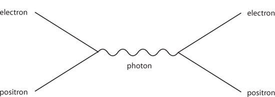
Here is a simple Feynman diagram. The way to think about this picture is that an electron and a positron (straight lines) come in from the left, meet each other, and annihilate into a photon (wavy line), which travels for a while before converting back into an electron/positron pair. There are specific rules that allow physicists to attach precise numbers to every such diagram, indicating the contribution that this picture makes to the overall process of “an electron and a positron scatter off each other.”
The story we tell based on the Feynman diagrams is just that, a story. It’s not literally true that an electron and a positron change into a photon and then change back. For one thing, real photons move at the speed of light, while electron/positron pairs (either the individual particles or the center of mass of a pair of them) do not.
What actually happens is that both the electron field and the positron field are constantly interacting with the electromagnetic field; oscillations in any electrically charged field, such as the electron or positron, are necessarily accompanied by subtle oscillations in the electromagnetic field as well. When the oscillations in two such fields (which we interpret as the electron and positron) come close to each other or overlap, all of the fields push and pull on one another, causing our original particles to scatter off in some direction. Feynman’s insight is that we can calculate what’s going on in the field theory by pretending that there are a bunch of particles flying around in certain ways.
This represents an enormous computational convenience; working particle physicists use Feynman diagrams all the time, and occasionally dream about them while sleeping. But there are certain conceptual compromises that need to be made along the way. The particles confined to the interior of the Feynman diagrams, which don’t either come in from the left or exit to the right, don’t obey the usual rules for ordinary particles. They don’t, for example, have the same energy or mass that a regular particle has. They obey their own set of rules, just not the usual ones.
That shouldn’t be surprising, as the “particles” inside Feynman diagrams are not particles at all; they’re a convenient mathematical fairy tale. To remind ourselves of that, we label them “virtual” particles. Virtual particles are just a way to calculate the behavior of quantum fields, by pretending that ordinary particles are changing into weird particles with impossible energies, and tossing such particles back and forth between themselves. A real photon has exactly zero mass, but the mass of a virtual photon can be absolutely anything. What we mean by “virtual particles” are subtle distortions in the wave function of a collection of quantum fields. Sometimes they are called “fluctuations” or simply “modes” (referring to a vibration in a field with a particular wavelength). But everyone calls them particles, and they can be successfully represented as lines within Feynman diagrams, so we can call them that.

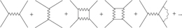
The diagram we drew for an electron and a positron scattering off each other isn’t the only one we could possibly draw; in fact, it’s just one of an infinite number. The rules of the game tell us that we should sum up all of the possible diagrams with the same incoming and outgoing particles. We can list such diagrams in order of increasing complexity, with subsequent diagrams containing more and more virtual particles.
The final number we obtain is an amplitude, so we square it to get the probability of such a process happening. Using Feynman diagrams, we can calculate the probability of two particles scattering off each other, of one particle decaying into several, or for particles turning into other kinds of particles.
An obvious worry pops up: If there are an infinite number of diagrams, how can you add them all up and get a sensible result? The answer is that diagrams contribute smaller and smaller amounts as they become more complicated. Even though there are an infinite number of them, the sum total of all the very complicated ones can be a tiny number. In practice, as a matter of fact, we often get quite accurate answers by calculating only the first few diagrams in the infinite series.
There is one subtlety along the way to this nice result, however. Consider a diagram that has a loop in it—that is, where we can trace around some set of particle lines to form a closed circle. Here is an electron and a positron exchanging two photons:
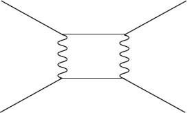
Each line represents a particle with a certain amount of energy. This energy is conserved when lines come together: if one particle comes in and splits into two, for example, the sum of the energies of those two particles must equal that of the initial particle. But how that energy gets split up is completely arbitrary, as long as the sum total is fixed. In fact, due to the wacky logic of virtual particles, the energy of one particle can even be a negative number, such that the other one has more energy than the initial particle did.
This means that when we calculate the process described by a Feynman diagram with an internal closed loop, an arbitrarily large amount of energy can be traveling down any particular line within the loop. Sadly, when we do the calculation for what such diagrams contribute to the final answer, the result can turn out to be infinitely large. That’s the origin of the infamous infinities plaguing quantum field theory. Obviously the probability of a certain interaction can be at most 1, so an infinite answer means we’ve taken a wrong turn somehow.
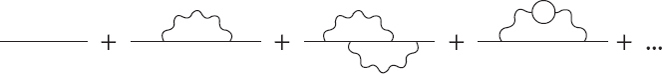
Feynman and others managed to work out a procedure for dealing with these infinities, now known as renormalization. When you have a bunch of quantum fields that interact with one another, you can’t simply first treat them separately, and then add in the interactions at the end. The fields are constantly, inevitably affecting one another. Even when we have a small vibration in the electron field, which we might be tempted to identify as a single electron, there are inevitably accompanying vibrations in the electromagnetic field, and indeed in all the other fields that the electron interacts with. It’s like playing a piano note in a showroom with many pianos present; the other instruments will begin to gently hum along with the original one, causing a faint echo of whatever notes you are playing. In Feynman-diagram language, this means that even an isolated particle propagating through space is actually accompanied by a surrounding cloud of virtual particles.
As a result, it’s helpful to distinguish between the “bare” fields as they would behave in an imaginary world where all interactions were simply turned off, and the “physical” fields that are accompanied by other fields they interact with. The infinities that you get by naïvely turning a crank in the Feynman diagrams are simply a result of trying to work with bare fields, whereas what we really observe are physical ones. The adjustment required to go from one to another is sometimes informally described as “subtracting off infinity to get a finite answer,” but that’s misleading. No physical quantities are infinite, nor were they ever; the infinities that quantum-field-theory pioneers managed to “hide” were simply artifacts of the very big difference between fields that interact and fields that don’t. (We face exactly this kind of issue when trying to estimate the vacuum energy in quantum field theory.)
Nevertheless, renormalization comes with important physical insights. When we want to measure some property of a particle, such as its mass or charge, we probe it by seeing how it interacts with other particles. Quantum field theory teaches us that the particles we see aren’t simple point-like objects; each particle is surrounded by a cloud of other virtual particles, or (more accurately) by the other quantum fields it interacts with. And interacting with a cloud is different from interacting with a point. Two particles that smash into each other at high velocity will penetrate deep into each other’s clouds, seeing relatively compact vibrations, while two particles that pass by slowly will see each other as (relatively) big puffy balls. Consequently, the apparent mass or charge of a particle will depend on the energy of the probes with which we look at it. This isn’t just a song and dance: it’s an experimental prediction, which has been seen unmistakably in particle-physics data.
The best way to think about renormalization wasn’t really appreciated until the work of Nobel laureate Kenneth Wilson in the early 1970s. Wilson realized that all of the infinities in Feynman-diagram calculations came from virtual particles with very large energies, corresponding to processes at extremely short distances. But high energies and short distances are precisely where we should have the least confidence that we know what’s going on. Processes with very high energies could involve completely new fields, ones that have such high masses that we haven’t yet produced them in experiments. For that matter, spacetime itself might break down at short distances, perhaps at the Planck length.
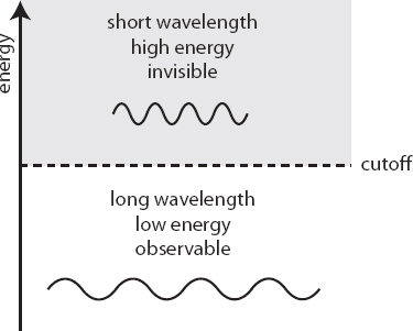
So, Wilson reasoned, what if we’re just a little bit more honest, and admit that we don’t know what’s going on at arbitrarily high energies? Instead of taking loops in Feynman diagrams and allowing the energies of the virtual particles to go up to infinity, let’s include an explicit cutoff in the theory: an energy above which we don’t pretend to know what’s happening. The cutoff is in some sense arbitrary, but it makes sense to put it at the dividing line between energies about which we have good experimental knowledge, and above which we haven’t been able to peek. There can even be a physically good reason to choose a certain cutoff, if we expect new particles or other phenomena to kick in at that scale, but don’t know exactly what they will be.
Of course, there could be interesting things going on at higher energies, so by including a cutoff we’re admitting that we’re not getting exactly the right answer. But Wilson showed that what we do get is generally more than good enough. We can precisely characterize how, and roughly by how much, any new high-energy phenomena could possibly affect the low-energy world we actually see. By admitting our ignorance in this way, what we’re left with is an effective field theory—one that doesn’t presume to be an exact description of anything, but one that can successfully fit the data we actually have. Modern quantum field theorists recognize that all of their best models are actually effective field theories.
This leaves us with a good news/bad news situation. The good news is that we are able to say an enormous amount about the behavior of particles at low energies, using the magic of effective field theory, even if we don’t know everything (or anything) about what’s happening at higher energies. We don’t need to know all the final answers in order to say something reliable and true. That’s a big part of why we can be confident that the laws of physics governing the particles and forces that make up you and me and our everyday environments are completely known: those laws take the form of an effective field theory. There’s plenty of room to discover new particles and forces, but either they must be too massive (high energy) to have yet been produced in experiments, or they interact with us so incredibly weakly that they can’t possibly have an effect on tables and chairs and cats and dogs and other pieces of the architecture of our low-energy world.
The bad news is that we would very much like to learn more about what’s really going on at high energies and short distances, but the magic of effective field theory makes that extremely hard. It’s good that we can accurately describe low-energy physics no matter what is going on at higher energies, but it’s also frustrating because this seems to imply that we can’t infer what’s going on up there without somehow probing it directly. This is why particle physicists are so enamored of building ever larger and higher-energy particle accelerators; that’s the only reliable way we know of to discover how the universe works at very small distances.