6 Stratification and fronts in shelf seas
Shelf seas in temperate latitudes undergo seasonal heating and cooling. We shall see in this chapter that this has an important effect on the structure of the water column, creating layering of the water in the summer. This, in turn, has implications for the biology of shelf seas, which are explored in Chapter 10.
6.1 The seasonal thermocline
On a summer’s day in a deep part of a temperate shelf sea where the tidal currents are not too strong, observations show that the water has thermal structure: it is divided into layers, with a surface layer of warm water lying on top of a deeper layer of cooler water (Figure 6.1). Immediately below the surface is a layer that is warmed by the sun and stirred by the wind, called the surface mixed layer, or the wind-mixed layer. Below this, the temperature decreases with depth, in a layer called the seasonal thermocline. Below the thermocline in shelf seas, there is usually another mixed layer (the bottom mixed layer) extending to the seabed. When the water is layered in this way it is said to be stratified.
The seasonal thermocline forms in early spring (late March or early April in the northern hemisphere). It develops first in the deeper parts of the shelf where the tidal currents are weakest. Around the British Isles these areas are in the northern North Sea and the Celtic Sea south of Ireland. The stratified area rapidly spreads into shallower water in the next few weeks, and at the same time it intensifies. Most of the sun’s heat now goes into the surface mixed layer, and so the temperature difference between surface and bottom of the water column increases. By midsummer, the temperature difference between the surface and bottom can be several degrees, with most of this occurring in just a few metres through the thermocline. After the summer solstice, the sea surface starts to cool, and at the same time wind speed tends to pick up as autumn approaches. The surface mixed layer now deepens and the thermocline is driven down towards the sea floor. This process transfers deep, cooler water into the surface mixed layer, lowering its temperature further. Eventually the water column becomes vertically mixed. This takes time, though, and the remnants of stratified water can linger in shelf seas in the northern hemisphere up until the beginning of December.
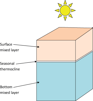
Figure 6.1 Illustration of a stratified water column, common in shelf seas in summer. A sun-warmed and wind-stirred surface mixed layer is divided from deep, cool tide-stirred water by a seasonal thermocline.
During winter, shelf seas cool, giving the summer warmth up to the atmosphere. The sinking of water cooled at the surface in convective overturning ensures that the water column remains vertically mixed until warming starts again in the following spring.
Even in summer, there will be parts of the shelf which remain immune to thermal stratification. These will include shallow water close to the coast (perhaps less than 10 m deep) where wind and waves together create enough turbulence to mix the sun’s heat from surface to seabed. In deeper water, tidal currents can be very effective at vertical mixing, and so regions with very fast tidal streams, for example near amphidromes (see Chapter 5) can remain vertically mixed throughout the year.
6.2 Stability and mixing in the thermocline
When the seasonal thermocline is present in the summer months it acts as a barrier to the vertical transport of material in the sea. This has important consequences for biology and sediment transport in shelf seas. In the spring, phytoplankton ‘bloom’ (or grow rapidly) in the well-lit surface mixed layer (more details of this are given in Chapter 10). This spring bloom strips nutrient salts out of the surface layer, but not out of the bottom layer, which is too dark for phytoplankton to grow. As a result, in the summer, the thermocline divides a welllit, but nutrient-depleted surface layer from a dark, but nutrient-rich bottom layer.
The reason why the thermocline acts as a barrier to vertical mixing can be understood if we remember the effect of temperature on water density (Chapter 2). Warm water is less dense than cold water. If we try and push some water from the surface mixed layer down through the thermocline it will be pushed back by its buoyancy (if you’ve ever tried to push a beach ball into the sea you will be familiar with this effect). Similarly, if we try to lift some water from the bottom mixed layer into the surface mixed layer, it will sink back down again because it is denser than the water into which it has been introduced (Figure 6.2). It is possible to mix water through the thermocline, but it takes energy to do so.
There are two principal sources of energy available for vertical mixing in shelf seas. These are provided by (a) the effects of the wind on the sea surface generating mixing in the surface mixed layer and (b) tidal streams rubbing against the sea floor generating mixing in the bottom mixed layer. It is these sources of energy that create the mixed layers, and they are also able to produce mixing between the layers (and hence across the thermocline) by a process called entrainment (section 6.4).
6.3 The thickness of the surface mixed layer
Figure 6.3 shows a useful way to envisage seasonal stratification in shelf seas. The surface mixed layer is warmed by the sun and stirred by the wind (depicted in this figure by a mechanical stirrer). The bottom mixed layer is stirred by the tide (depicted by another mechanical stirrer) and a thermocline separates the two layers. We can then use a simple, but rather elegant, energy model to show how the thickness of the surface mixed layer depends on the wind speed and the rate of warming by the sun.
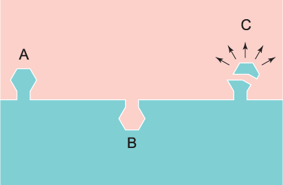
Figure 6.2 The thermocline barrier. Warm surface water is coloured pink and cold bottom water blue. An intrusion of cold water into the upper warm layer, as at A, will sink back down again because it is denser than the surrounding warm water. Similarly, an intrusion of warm water downwards (at B) will rise back because it is buoyant. It is only if the intrusion is given enough energy to overcome the density difference that transfer of water across the thermocline can take place. In the example at C, cold bottom water is being entrained into the surface layer.
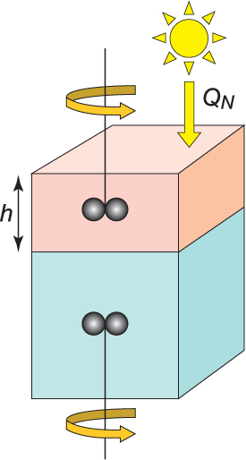
Figure 6.3 Heating–stirring model of the seasonal thermocline. The sea is heated by the sun (at a net rate QN) and stirred at the surface by the wind and at the bottom by the tide (stirring is represented here by turning paddles). Wind stirring drives the thermocline down and tidal stirring drives it up. The resulting position of the thermocline (and the thickness of the layers) depends on the balance between these two processes.
As the surface layer is warmed by the sun it expands, and therefore its potential energy increases as its centre of gravity rises. It can be shown that the rate of increase of the potential energy of the surface mixed layer is proportional to its thickness times the net rate of heating (that is the solar flux of heat through the surface minus the heat losses back to the atmosphere). If we call the thickness of the surface mixed layer h and the net rate of heating QN, then the rate of increase of potential energy is proportional to the product hQN. Now, the rate at which the wind puts energy into the sea is proportional to the cube of the wind speed (this is because the friction force of the wind on the sea depends on the square of the wind speed, and the rate of work done by this force is equal to the force times the wind velocity). Most of the energy put into the sea by the wind is dissipated as heat or used to make waves, but a small fraction (less than 1 %) is utilised in mixing the sun’s heat down and creating the surface mixed layer. Let’s suppose that a constant fraction of the wind energy is used for this purpose. Then the energy available from the wind to create the surface mixed layer is proportional to w3 where w is the wind speed. In steady state, the energy input just balances the energy increase and something that is proportional to w3 is equal to something that is proportional to hQN. That is

where C is a constant. Experiments show that if h is expressed in metres, w in m s–1 and QN in Wm–2 then C is about equal to 8.
The equation above can be used to estimate the thickness of the surface mixed layer if the wind speed and heat flux through the sea surface are known. The latter can be estimated from changes in temperature of the water. If the water is warming up, this implies a positive heat flux through the surface. If the water is cooling down, the sea is giving heat back to the atmosphere. Table 6.1 below shows estimates of QN, calculated in this way, for a fixed observatory station (station E1) in the English Channel, operated by Plymouth Marine Laboratory. Notice that the net heat flux is positive for six months (the sea is warming up) and negative for the other six months. The table also shows monthly mean wind speeds measured at Aberporth on the Welsh coast. The depth of the surface mixed layer, calculated from the equation, is also shown.
Table 6.1: Estimates of the net rate of heating (QN), calculated for a fixed observatory station (station E1) in the English Channel operated by Plymouth Marine Laboratory. h is the height of the mixed layer depth and w is the wind speed.
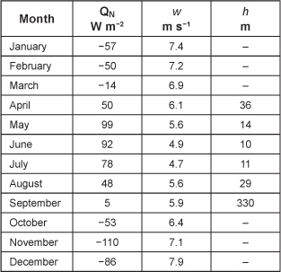
Notice that a mixed layer depth cannot be calculated when QN is negative. A surface mixed layer will only form when the surface is being heated. When it is being cooled, convection will overturn the water column and the mixed layer depth will be the same as the water depth. Notice also that for September, a surface mixed layer depth of 330 m is calculated. Since the total water depth here is only about 50 m, this means that actually the water column will be well mixed in this month, even though it is still being heated weakly at the surface.
6.4 Entrainment
The surface mixed layer deepens in the autumn months through the process called entrainment. The turbulence generated in the surface layer by the wind produces undulations (or internal waves, see Chapter 2) in the thermocline. If these become sufficiently vigorous, the tops can break off, transferring parcels of water from the lower into the upper layer. Entrainment always takes place from relatively still water towards more vigorously stirred water. The entrained water makes the volume of the surface layer increase (and that of the bottom layer decrease) and as a result the thermocline moves down at a speed called the entrainment velocity. The entrained water transfers material from the bottom layer into the surface layer. For example, it will transfer nutrients that are needed by phytoplankton (Chapter 10).
At the same time as entrainment into the surface layer is occurring, stirring in the bottom layer by tidal mixing entrains surface water into the bottom mixed layer. Since the surface water is warmer, this produces a warming of the bottom mixed layer, which can be observed in records of bottom water temperature (Figure 6.4).
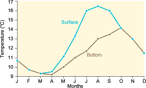
Figure 6.4 Annual variations in surface and bottom temperature at station E1 in the English Channel.
It is possible to work out the entrainment velocity due to tide mixing from the rate of warming of the bottom layer. The entrainment velocity is equal to this rate of warming multiplied by the thickness of the bottom layer and divided by the temperature difference between the surface and bottom layers. The thickness of the bottom layer at station E1 in summer is about 30 m. The rate of warming of the bottom layer (from Figure 6.4) in summer is about 5 °C in 6 months or about 0.03 °C per day. In June, the temperature difference between top and bottom is about 2 °C. These figures give an entrainment velocity of about 0.5 m per day. The thermocline will not necessarily move upwards at this speed because wind mixing is driving it downwards at the same time. The net rate of movement of the thermocline will be the difference between the upwards entrainment velocity due to the tide and the downward entrainment velocity due to the wind. It is possible to have a situation in which the thermocline is not moving, but water is being entrained across it at equal rates by wind and tidal stirring.
6.5 Tidal mixing fronts
If the combined stirring by wind and tide is sufficiently vigorous, it can prevent the seasonal thermocline forming altogether, and the water remains vertically mixed throughout the year. This happens in large parts of the north-west European shelf where the tidal currents are fast, including much of the Irish Sea, the English Channel and the southern North Sea. In other places, where the tidal streams are not so fast, a seasonal thermocline forms in the summer. The places where the transition occurs between vertically mixed and stratified water are called tidal mixing fronts (Figure 6.5).
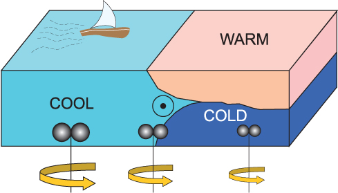
Figure 6.5 A tidal mixing front divides stratified and vertically mixed water in the summer in shelf seas. At the surface the front is characterised by a transition from warm to cool water. The turning paddles show the weakening gradient of tidal stirring in the direction of the stratified water. The dotted circle at thermocline depth at the front represents the current flowing along the front (see section 6.7).
On one side of the front, the water is thermally stratified, with warm water lying on top of cold. On the other side of the front, the water is vertically mixed, with uniform cool water from sea surface to the seabed. There are often changes in water colour and transparency, which are noticeable to viewers on a ship or aeroplane crossing the front (figure 6.6). There is also a difference in surface temperature. For this reason, tidal mixing fronts are visible from space in thermal infra-red imagery (Figure 6.7).
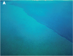
Figure 6.6 (A) Aerial photograph of a tidal mixing front (the one marked C in Figure 6.6). The stratified water is to the right of the front and is a clearer blue compared to the mixed water to the left of the front.
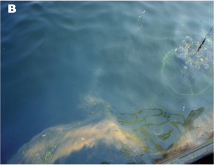
Figure 6.6 (B) Water surface view of front showing a CTD rosette sampling directly under the front interface where phytoplankton, feathers and even some seaweed are accumulating.
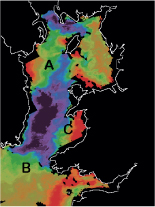
Figure 6.7 Satellite infrared image of the Irish Sea showing sea surface temperature. Cool surface waters are shown in purple and blue, and warm waters in green, yellow and red. Sharp gradients in sea surface temperature marked at A, B and C are associated with tidal mixing fronts.
Unlike weather fronts in the atmosphere, tidal mixing fronts form in the same places each year. This is because their position is controlled by the geographical distribution of the strength of the tidal streams, and this doesn’t change with time: places that have strong tidal currents always have strong tidal currents.
We can derive a criterion for the location of fronts using an extension of the energy argument of section 6.3. For water to be vertically mixed, there has to be a sufficient supply of stirring energy to provide the increase of potential energy due to thermal expansion. For a vertically mixed water column of depth h, the rate of increase of potential energy as it is heated at net rate QN is proportional to hQN. The rate at which energy is supplied by the wind is proportional to the cube of the wind speed. Similarly, the rate at which energy is supplied by the tide is proportional to the cube of the tidal current speed. Equating the rate of supply of stirring energy to the rate of increase of potential energy gives:
au 3 + bw 3 = hQN
In fact, as their name suggests, most of the energy at tidal mixing fronts is provided by the tide, and so we can neglect the second term in this equation in comparison with the first. If the stirring is not provided at a sufficient rate, i.e. au3<hQN, complete vertical mixing cannot be maintained and the water column responds by becoming stratified (the rate of increase of potential energy immediately becomes less because only the surface mixed layer is expanding now). Exactly at a tidal mixing front, therefore,
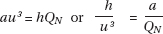
QN doesn’t change too much from place to place in a given shelf sea area, and so effectively fronts will occur along lines where h/u3 = constant. Tidal mixing fronts will form at places in the sea where the water depth divided by the cube of the current speed is equal to a certain value. If u is taken as the maximum surface tidal current speed at spring tides, the value of the constant appears to be about 70. So if the water depth is 70 m, we would expect a tidal mixing front to occur along a line where the maximum current is about 1 m s–1. Places where the current is weaker than this would be stratified, and places where the currents are stronger would be vertically mixed.
In the Irish Sea, where tidal mixing fronts were first studied, the front runs from the southern tip of the Isle of Man towards the east coast of Ireland (the western Irish Sea front). This separates mixed water to the east (where the tidal currents are strong) from stratified water to the west (where the currents are weak). The other main tidal mixing fronts around the UK are one stretching across the southern entrance to the Irish Sea (the Celtic Sea front), one off the west coast of Scotland (the Islay front), and a long one stretching across the North Sea (the Flamborough Head front). In addition, tidal mixing fronts have been discovered in many shelf sea regions of the world, including George’s Bank in Canada, Cook Strait in New Zealand and the Patagonian Shelf in South America.
6.7 Dynamics of tidal mixing fronts
It would be difficult to make the structure shown in Figure 6.5 in a laboratory tank. The warm surface water will tend to spread out towards the left (and the cold bottom water will also tend to spread out along the bottom, also towards the left in the figure). In the sea, this is prevented from happening by the Coriolis effect (Chapter 4). The warm surface water initially spreads out, but then turns to the right (in the northern hemisphere) under the influence of the Earth’s rotation. The same thing happens to the cold bottom water. This effect creates currents flowing along the front.
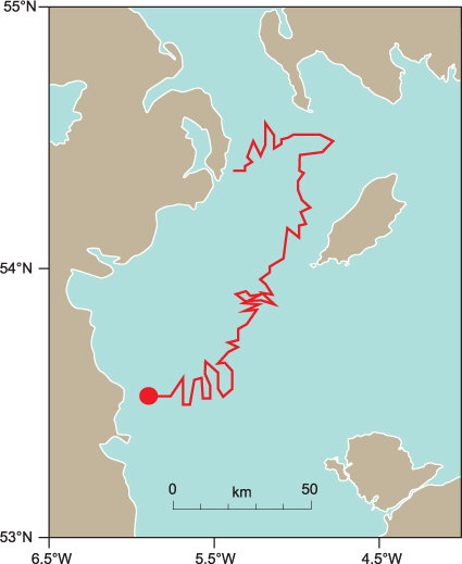
Figure 6.8 Paths of satellite tracked buoys in the Irish Sea. The buoys flow along the front in this part of the Irish Sea, travelling on an anticlockwise circuit known as the gyre.
In fact these flows also create a surface slope, and the flow then adjusts so that there is a single current flowing along the front at the depth of the thermocline, at speeds of a few tens of centimetres per second. This flow travels with the stratified water on its left looking along the direction of flow. Because this flow is weak compared to the tidal streams at the front, it is difficult to detect with conventional current meters. It can, however, be detected with Lagrangian techniques using satellite-tracked drifters fitted with an underwater sail (or drogue) at thermocline depth. In the western Irish Sea front, such drifters flow along with the stratified water on their left and can perform complete circuits of the stratified water in the western Irish Sea (Figure 6.8). For this reason, this part of the Irish Sea is sometimes called the gyre.
We have seen that tidal mixing fronts form along lines where the value of the water depth divided by the tidal current cubed (h/u3) is constant. The strength of the tidal streams, u, changes with the springs/neaps cycle, and as this happens, the front tries to adjust its position so it remains at the critical value of h/u3. This movement is called the springs/neaps adjustment of fronts. At spring tides, some of the stratified water adjacent to the front becomes mixed and the front advances into the stratified water. At neap tides, some of the mixed water adjacent to the front becomes stratified and the front moves back again.
This movement can be observed from space. It is not large – just a few kilometres – but as the front moves back and forth in this way, water is transferred from the high-nutrient mixed water into the low-nutrient stratified water. It is thought that this process may account for some of the high biological productivity observed at these tidal mixing fronts.