10  Primary production in the oceans

As stressed before in previous chapters, the fundamental process underlying all of the marine foodwebs is the production of organic matter through photosynthesis by the phytoplankton and some members of the picoplankton. The amount of new biomass that is made by the photosynthetic organisms (primary production) ultimately determines the size of zooplankton, fish, whale and seabird stocks, as will be discussed in Chapter 11. So understanding the factors controlling primary production in the oceans is of primary importance in our understanding of the management and utilisation of the biological resources of the oceans.

10.1 Photosynthesis and respiration

In the oceans there are very few plant species. Seaweeds, which cover many intertidal shores and grow down to 50 m or so in the subtidal zone, look as though they should be classified as plants. However, they are in fact algae (macroalgae or large algae). Although they photosynthesise, they differ from plants in that they do not flower and have no roots, leaves or highly organised tissues for transporting water and nutrients. The only true plants in the oceans are a relatively small group of the sea grasses. The unicellular algae of the phytoplankton are related to the seaweeds and termed microalgae (or microscopic algae).

These issues aside, the photosynthetic plankton can photosynthesise in the same way that terrestrial plants do, in that they use light as their energy source and carbon dioxide to produce new organic matter, a consequence of which is the production of oxygen. The photosynthetic process can be divided into two: a light reaction and a dark reaction. The light reaction converts light into metabolic energy and reducing power. Specialised light sensitive pigments such as chlorophylls absorb light energy, which is subsequently used in the dark reaction to reduce (fix) CO₂ to organic compounds (generally symbolised as CH₂O). The overall reactions are:

Light reaction: 2H₂O + light ⇒ 4[H⁺] + metabolic energy + O₂

Dark reaction: 4[H⁺] + metabolic energy + CO₂ ⇒ [CH₂O] + H₂O

Generally photosynthesis (combining light and dark reactions) is represented by the following equation:

6CO₂ + 6H₂O + 48photons of light ⇒ 6O₂ + C₆H₁₂O₆

The most common pigment used by phytoplankton, as in plants, to trap light is chlorophyll a (Chla), which absorbs blue (maximally at 430 nm) and red wavelengths (maximally at 680 nm) of light and reflects green wavelengths (the reason why plants look green). However, there is a large variety of other chlorophylls and other pigments that are used in different species to absorb other wavelengths of the PAR (400 to 700 nm, see Chapter 7): Carotenoids such as b-carotene and fucoxanthin, as well as chlorophyll-b, absorb in the green part of the light spectrum (400 to 520 nm), whereas phycoerythrin absorbs in a different range of the green region (490 to 570 nm). Phycocyanins and allophycocyanins absorb light in the green–yellow (550 to 630 nm) and orange–red (650 to 670 nm) parts of the spectrum respectively. These pigments are examples of accessory pigments, and phytoplankton adjust the composition and concentrations of their light harvesting pigments to absorb various components of the PAR spectrum of light as it varies with water depth. So a phytoplankton cell in well illuminated surface water will have a different composition of pigments than that found near the bottom of the photic zone. Additionally, as phytoplankton move from a high light to a region of low light they synthesise more chlorophyll and pigments to be able to maximise the harvesting of photons. Conversely when moving from low light to high-light conditions they tend to decrease the concentration of chlorophyll and other pigments inside the cells. Some of accessory pigments are very effective at screening out ultraviolet (UV) parts of the light spectrum (which can cause immense damage to cells), and often in high-light environments UV screening pigments are very rapidly produced.

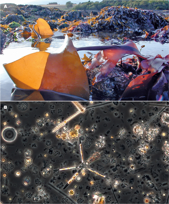
Figure 10.1 (A) Seaweeds are macroalgae which are related to (B) Phytoplankton. Both are not plants but are algae.

The other essential metabolic pathway for life to proceed is respiration. All organisms respire to produce energy, and unlike photosynthesis, which can only take place in the light, respiration takes place continuously; but critically it is dependent on there being oxygen present. Effectively the equation for respiration is the reverse of that for photosynthesis: 6O₂ + C₆H₁₂O₆ ⇒ 6CO₂ + 6H₂O + energy The amount of energy produced is highly dependent on the nature of the starting material: for a given weight of material, the respiration of lipids (fats) produces at least twice as much energy as carbohydrates (sugars), which is why fats are widely used as a storage material in all groups of life.

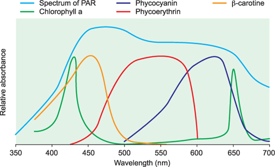
Figure 10.2 Spectrum of PAR with absorption spectra of chlorophyll and other pigments sketched in.

10.2 Phytoplankton growth

A phytoplankton cell is not just composed of the carbohydrates generated by photosynthesis, but is made up of cell walls, membranes, proteins, enzymes, etc. So as well as photosynthesis taking place, inorganic nutrients such as nitrogen, phosphorus, and sulphur need to be assimilated to build the complexity of life. The total list of elements that are needed is enormous, although some of these are required in minute or trace amounts. As a very crude estimation, a functioning phytoplankton cell comprises around 40% protein, 5% nucleic acids and nucleotides, 40% carbohydrates, and 15% lipids. This allows us to rewrite the simplified photosynthesis equation to take into account the need for nitrogen and phosphorus:

106CO₂ + 16NO₃^– + HPO4₂^– +122H₂O + 18H⁺ ⇒ C₁₀₆H₂₆₃O₁₁₀N₁₆P + 138O₂

From the equation above we can derive the ratio of carbon: nitrogen: phosphorus in healthy, actively growing algal cells as 106:16:1. This ratio is the same as the Redfield ratio (after the American oceanographer A.C. Redfield) which describes the elemental composition of the bulk of the particulate organic matter in the oceans. The C : N ratio in the above is 6.6 : 1, which is a commonly used measure to determine the physiological status of algae, since when nitrogen is limited, or the algal cells are senescent or dying, this ratio increases considerably.

10.3 Photosynthesis and light

The relationship between photosynthesis and light (irradiance) is described by a photosynthesis/irradiance curve (P/I curve, Figure 10.3). It is important to remember that although photosynthesis is light-dependent, respiration is constant. With increasing light, photosynthesis increases linearly (with a slope of a) until it reaches a particular irradiance where the photosynthetic rate is equal to the respiration rate. This point is called the compensation irradiance, I_c. The irradiance where this occurs is species specific, and even within a single species can vary seasonally or on even shorter timescales.

As irradiance increases further, the trend becomes gradually non-linear and a point is reached where further increases in irradiance do not result in increases in the photosynthetic rate. In other words, the rate of photosynthesis is light saturated, and the maximum rate of photosynthesis (P_max) has been reached. The saturation irradiance I_k is the irradiance at the intercept of the two lines shown in figure 10.3. In some organisms, there is a decrease in photosynthetic rates at very high irradiances (photoinhibition) resulting from damage to cell membranes or proteins.

Two other important terms need to be noted: gross photosynthesis is equivalent to the total photosynthesis, and net photosynthesis is equal to gross photosynthesis minus respiration. The distinction between these is pertinent, since it is only really the net photosynthetic energy gains that are available for cell growth and reproduction.

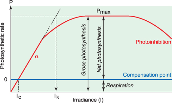
Figure 10.3 Photosynthesis vs. Irradiance curve (P/I curve).

10.4 Photosynthesis and growth

By comparing what we know about how light decreases through the photic zone, and coupling this with the information of the P/I curve, it is possible to describe the trends in photosynthesis in the surface oceans. If a cell could maintain its position at the very surface of the water, naturally this is the maximum light available for optimum photosynthesis to occur. If it is at the bottom of the photic layer (1% of incident light), there may still be enough light for photosynthesis to occur, but potentially not enough to reach or surpass the compensation point. There will be a point in the water column, the compensation depth, at which the gross photosynthetic carbon assimilation by the phytoplankton equals the respiratory carbon losses, or when the net photosynthesis is 0 (equivalent to I_c on the P/I curve).

However, phytoplankton cells are not static in the water, since they are sinking and being mixed either throughout the whole water column or, where water stratification takes place, within surface mixed water layers (Chapter 3). The depth of the mixed layer may be below that of the compensation depth, and so when considering net phytoplankton growth it is more pertinent to relate the daily integrated photosynthetic gains to the integrated respiration losses over the water column (day and night) to the depth of the mixed layer.

The critical depth is the water depth where the integrated daily photosynthetic carbon assimilation is balanced by the integrated daily respiratory carbon losses. As long as sufficient nutrients are present, net phytoplankton growth occurs when the mixed layer depth is shallower than the critical depth. When the mixed layer extends below the critical depth algal growth is limited by light, and there is no net phytoplankton growth.

If the water is so turbid that very little light reaches the bottom of the mixed layer, it can be shown that the mean irradiance experienced by the cell is equal to I₀/(kh), where I₀ is the surface irradiance, h is the depth of the mixed layer and k is the attenuation coefficient. If this mean irradiance is greater than the I_c for the cell, then it can grow in the surface mixed layer.

In the spring, the seasonal thermocline becomes established in the sea in temperate latitudes, trapping phytoplankton in a relatively shallow surface mixed layer (see Chapter 6). At the same time, the surface light levels are increasing. As a result of the increasing surface irradiance (I₀) and the decreasing depth of the surface mixed layer (h), the mean irradiance in the surface mixed layer increases sharply in the spring (Figure 10.4). Often, a clearing of the water in the surface layer as suspended sediment sinks out, reducing the attenuation, will also help to increase mean irradiance in the surface layer. The spring bloom, when phytoplankton start to grow rapidly, producing a visible greening of the water, begins when the mean irradiance in the surface mixed layer exceeds the compensation irradiance.

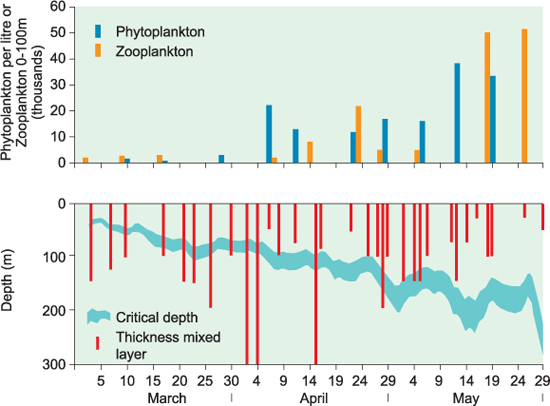
Figure 10.4 Data from the Norwegian Sea in 1949 showing the relationship between mixed layer depth, critical depth, and phytoplankton and zooplankton abundance. Growth of phytoplankton only occurred when the depth of mixing was consistently above the critical depth. (Illustration adapted from Sverdrup’s original data).

Example calculation of the timing of the spring bloom

As a quantitative illustration of the occurrence of the spring phytoplankton bloom, suppose that the compensation irradiance for a certain phytoplankton group has a value of 20 µE m²s^–1. Let the depth of the surface mixed layer be 30 m and the diffuse attenuation coefficient be 0.5 m^–1. If the surface irradiance is I₀, then the mean irradiance in the surface mixed layer will be I₀/(0.5*30) = I₀/15. The spring bloom will start on the day on which this mean irradiance first exceeds the compensation irradiance, that is I₀/15>20, from which it follows that I₀>300 µE m^–2s^–1. If these conditions were occurring at the latitude of Dunstaffnage, we would expect the spring bloom to start in the middle of April (see figure 7.4).

10.5 Nutrients limiting phytoplankton growth

Phytoplankton growth can only carry on as long as all the nutrients are present in adequate supply, and seasonal algal blooms are normally brought to an end when a nutrient (normally phosphorus or nitrogen) becomes used up. In the scenario described above for temperate shelf seas, nutrients are returned to surface waters in autumn and winter once the thermocline breaks up and the nutrient-depleted surface waters are able to mix with the nutrientrich deeper layers. If there is enough light still around when this breakdown of the thermocline begins (which can sometimes be the case in autumn) there may be a second short bloom of phytoplankton.

Generally we talk about nitrogen or phosphorus limiting phytoplankton growth; however, it may not be the lack of one of these major nutrients that stops the growth, but rather one of the nutrients needed in only trace amounts. There are some ocean waters where phytoplankton growth is never sufficient to deplete the nitrogen and phosphorus in surface waters. These are known as highnutrient, low-chlorophyll (HNLC) waters, and are located in the subarctic Pacific, the Southern Ocean, and the equatorial Pacific. What is common for all of these is that they are relatively far away from land. Iron is an essential element for several metabolic processes in phytoplankton cells, but it turns out that these waters have remarkably low concentrations of dissolved iron. The primary source of iron to the surface waters of the oceans is from the land, either directly or via deposition of dust from the atmosphere. Over the past 20 years there have been a number of large-scale experiments in several HNLC regions where dissolved iron has been added to the surface waters, and these have all resulted in spectacular phytoplankton growth. So although only needed in trace amounts, the iron is clearly the limiting nutrient in these systems.

As we have discussed, in stratified waters, algal growth in the upper mixed layer can deplete the nutrients to the point where further growth is not possible. However, a commonly observed phenomenon in such circumstances is a layer at, or just above, the thermocline where phytoplankton growth is still taking place. These layers are called sub-surface chlorophyll maxima, and form when the boundary between the surfacemixed waters (nutrient-depleted) and lower water mass (nutrient-replete) is above the critical depth. Nutrients from waters below the boundary layer diffuse upwards, aided by small-scale turbulence, into the thermocline region. Phytoplankton entrained in this zone are able to use the nutrients since there is still enough light for net growth to take place.

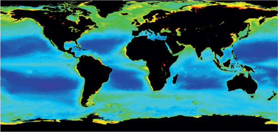
Figure 10.5 Chlorophyll distribution in surface waters of the oceans. Note the large areas in the subarctic Pacific, the Southern Ocean, and the equatorial Pacific where productivity is low, the so-called nutrient low chlorophyll (HNLC) regions regions; c.f. figures 9.8 & 9.9..

This is an example of how phytoplankton growth is being stimulated by the coming together of two water bodies with different physical and chemical properties. The surface waters are stabilised, warm and well lit, but lack nutrients, and the waters below the thermocline are cold and dark but do have nutrients. Therefore at the front between the water layers the two water bodies complement each other to provide conditions favourable for primary production to take place. Similar complementation effects are seen at other frontal systems in shelf seas, such as tidal fronts or shelf-sea fronts, and fronts associated with river/estuarine plumes.

There are several coastal regions, notably off Peru, Chile, south and north-eastern coasts of Africa, where winds blowing parallel to the coastline result in the transport of nutrientdepleted surface waters away from the land. This is replaced by nutrient-rich water from below (upwelling), the consequence of which is that these regions support the highest primary production, and in turn zooplankton and fish production, on Earth.

Upwelling of nutrient-rich waters also occurs at major ocean frontal systems in the open oceans, such as the equatorial regions in the Pacific Ocean where the trade winds generate two westerly flowing surface currents, the North and South Equatorial Currents. The Coriolis effect causes the currents to deflect northwards in the northern hemisphere and southwards in the southern hemisphere. The divergent flow of these surface waters away from the Equator causes nutrient-rich water to upwell to the surface, supporting higher rates of primary production than that in adjacent waters. Cyclonic gyres found in several regions (anticlockwise in the northern hemisphere and clockwise in the southern hemisphere) also result in nutrient-rich waters being upwelled from below the thermocline into surface waters as a result of the Coriolis effect producing slopes in the pycnocline, as described in section 4.4. Higher rates of primary production are a consequence of this nutrient exchange.

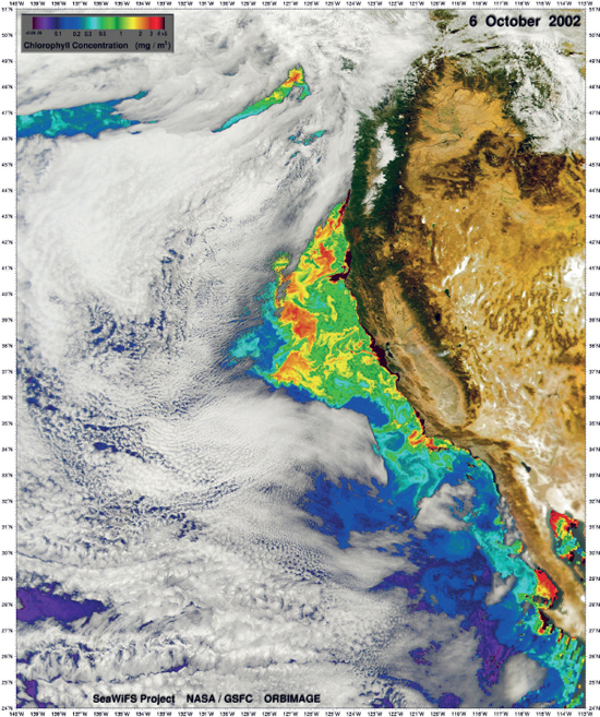
Figure 10.6 Upwelling of nutrient-rich waters off the coast of California causes increased primary production as revealed by this satellite image of surface chlorophyll concentrations.

10.5 Primary production on a global scale

Trying to classify annual primary production of all the oceans is of course difficult, but remote sensing techniques have enabled us to make good estimations of the regional differences (Figure 10.7). It is quite evident that as well as upwelling regions, the coastal waters and epipelagic overlying continental shelves also support the greatest primary productivity.

It would be expected that due to the good light conditions in tropical and sub-tropical oceans, these regions would be highly productive. However, this is not the case, since there is normally a permanent thermal stratification, which means that there is no mixing with deeper waters for long periods of time, and the upper mixed layers are generally depleted in major nutrients. In complete contrast, in the polar oceans there is generally significant exchange of nutrient-rich lower waters with the surface waters, and these regions are characterised by long periods of low light and sea-ice cover which severely limits primary production. However, when the light does come, day lengths are long and sun angles high, so there tend to be short but intense periods of primary production in the Arctic and Southern Oceans, although remembering that the latter is an HNLC region and iron limited.

In conclusion, estimates of the net primary productivity of the global ocean range between 40 and 50 Pg carbon year^–1 (P = peta, and 1 Pg is equivalent to 10¹⁵ g). This value is remarkably similar to the estimates of total land-based primary production. In other terms, the productivity of algae and photosynthetic bacteria in the top 200 m of the oceans equals that of ALL the vegetation in the forests, grasslands and crops on land.

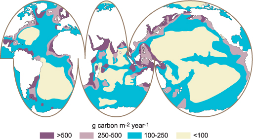
Figure 10.7 The annual primary production of the oceans from a global perspective.