2
The atomic nucleus
Radioactivity was discovered by Antoine Henri Becquerel in 1896. He found that the mineral crystal he was investigating caused a photographic plate to become blackened. It was an accidental discovery because he had been looking for the emission of X-rays from the crystal; X-rays had also recently been discovered. However, the crystal happened to contain some uranium, which produced the nuclear radiation. There followed a period of intense research on the nature of this radiation and the materials that emitted it. Marie and Pierre Curie isolated and identified the radioactive element radon, while Ernest Rutherford found three distinct forms of nuclear radiation, which he characterised by their ability to penetrate matter and ionise air. The first type of radiation, which penetrated the least, but caused the most ionisation, he called alpha (α) rays. The second type, with intermediate penetration and ionisation, he called beta (β) rays, and the third type, which produced the least ionisation but penetrated the most, he called gamma (γ) rays. It was subsequently discovered that α-rays are composed of helium nuclei, β-rays are composed of electrons and γ-rays are composed of high-energy photons. Becquerel, the Curies and Rutherford all received Nobel prizes for their discoveries. A turning point in the understanding of the atomic nucleus came in a series of pioneering experiments by Rutherford and his collaborators at the University of Manchester. They directed a beam of α particles at a thin gold foil and observed how the α particles were deflected by the foil. Based upon their observations, Rutherford postulated a model of the atomic nucleus that remains familiar today: a model in which all the positive charge of the atom and all the mass is concentrated in an extremely small region called the nucleus. It could be said that nuclear physics began with Rutherford's discovery of the atomic nucleus.
In parallel with these experiments on the atomic nucleus there were the revolutionary developments of quantum mechanics and relativity. These considerably aided the understanding of the results of the experiments, and indeed these experiments provided convincing evidence for the validity of the new theories. In 1905 Einstein published his equation describing the equivalence of mass and energy:

Einstein's equation shows that huge amounts of energy are released when mass–energy conversion takes place, as happens in nuclear fission and nuclear fusion. The fission of heavy nuclei, such as uranium, is a major source of power today, while the fusion of light nuclei is the energy source that powers the stars, including our Sun, and has the potential to play a key role in providing the energy needs of the future. Nuclear fission and nuclear fusion are discussed in Chapter 3.
In this chapter we describe the composition of nuclei and their basic properties, including their size, mass and electric charge. The characteristics of the forces that bind the constituents of a nucleus together are also described together with the resulting nuclear binding energies. We will see how the binding energy is intimately related to the energy that we can obtain from nuclear fission and fusion through the equivalence of mass and energy. We will also see that binding energy plays a central role in the stability of nuclei and that unstable nuclei decay to more stable nuclei. The various ways in which radioactive decay can occur will also be described.
2.1 The composition and properties of nuclei
2.1.1 The composition of nuclei
At the centre of an atom is a positively charged nucleus. The nucleus is very small compared with the overall size of the atom; an atomic diameter is ∼10− 10 m, while the diameter of a nucleus is ∼10− 14 m, a factor of ∼104 smaller. The nucleus contains just two kinds of particles, protons and neutrons. Protons and neutrons are much heavier than electrons, by a factor of approximately 2000, and so nearly all the atomic mass is concentrated in the nucleus. A nucleus is characterised by the number of protons and neutrons it contains. The number of protons is called its atomic number Z. Since a proton has a charge +e, where e is the magnitude of the electronic charge, the nuclear charge is equal to +Ze. The number of atomic electrons must be equal to the number of protons in the nucleus to maintain charge neutrality, and so an electrically neutral atom must therefore have Z electrons. The number of neutrons a nucleus contains is called its neutron number, N. A neutron has a mass that is very close to that of a proton, but it is electrically neutral. The proton and neutron are collectively known as nucleons, as they are both found in the nucleus. The total number of protons and neutrons is called the nucleon number, A, which is more usually called the mass number or atomic mass number of the nucleus. (This follows, as nuclear masses are measured on a scale in which the proton and the neutron have masses that are close to one fundamental unit of mass. A is then the integer nearest to the ratio between the nuclear mass and the fundamental mass unit.) A particular species of nucleus is called a nuclide and is specified by its values of A, Z and N as:
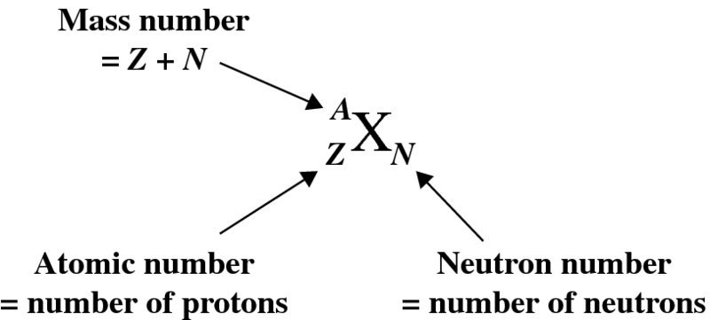
where X is the chemical symbol. An example is 5828Ni30, pronounced nickel-58. Note that we do not need to write both the chemical symbol and the atomic number because the chemical symbol tells us the value of Z; for example, every nickel atom has Z = 28. It is also usually not necessary to include N, as N = A − Z. Thus we can simply and conveniently write AX; for example 58Ni. (Including Z and N is useful when we are trying to balance Z and N in a nuclear reaction or decay process.)
Naturally occurring samples of most elements contain atoms with the same atomic number
Z but with different values of mass number A. Nuclides with the same Z but different N are called isotopes. Typically an element may have two or three stable isotopes, although some, like
gold, have just one while iodine has nine. A familiar example is chlorine (Z = 17). About 76% of naturally occurring chlorine nuclei have N = 18, while 24% have N = 20. These fractions are called the natural abundances of the respective isotopes. The chemical properties of an element are determined
by its atomic electrons. As different isotopes of the same element have the same number
of electrons, they have the same chemical properties. On the other hand, different
isotopes have slightly different physical properties – in particular, properties that
depend on mass. For example, the
 and
and
 isotopes of uranium can be physically separated because of the slightly different
diffusion coefficients of the gases
isotopes of uranium can be physically separated because of the slightly different
diffusion coefficients of the gases
 F6 and
 F6. This has important application in enriching naturally occurring uranium for nuclear
fission reactors.
F6. This has important application in enriching naturally occurring uranium for nuclear
fission reactors.
2.1.2 The size of a nucleus
A measure of nucleus size was first obtained by Rutherford and his collaborators, Hans Geiger (inventor of the Geiger counter) and Ernest Marsden, the latter still being an undergraduate student at the time. Rutherford had already established that α particles are doubly ionised helium atoms, He++, where both electrons have been removed from the atom. He then used α particles as a probe of the nucleus. In these experiments, beams of α particles were fired at thin metal foils and the way these particles were deflected or scattered by the foils was investigated. (Firing energetic projectiles at sub-atomic particles remains, of course, a principal means of investigating their nature.) These investigations culminated in Rutherford's model of the structure of the atom: all the positive charge of the atom, and consequently all the mass, is concentrated in an extremely small region called the nucleus.
The Rutherford scattering experiment
A schematic diagram of the apparatus for Rutherford's scattering experiment is shown in Figure 2.1. The radioactive source emits α particles of well-defined kinetic energy E. This energy is typically about 5 MeV1 and is measured in a separate experiment by observing the motion of the α particles in crossed electric and magnetic fields. The α particles are collimated into a narrow beam using a combination of apertures and are directed onto a thin gold foil. The foil is so thin that most of the α particles pass through it with little energy loss. However, the charged α particles suffer deflections because of their electrostatic interactions with the positive and negative charges in the gold atoms, although the electrons are so light that they do not deflect the α particles appreciably. The scattered α particles are detected on a flourescent screen that produces a tiny flash of light when an α particle strikes it. In this way it is possible to measure the angular distribution of the scattered α particles, i.e. the number of detected α particles as a function of scattering angle θ.
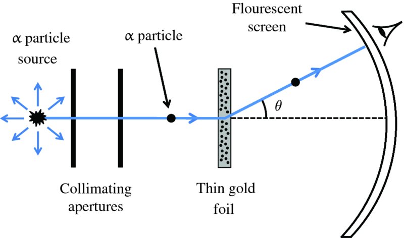
Figure 2.1 Schematic diagram of Rutherford's apparatus for observing the scattering of α particles by a thin gold foil. α particles from the source are collimated into a narrow beam and directed at the foil. The angle θ through which an α particle is deflected at the foil is measured by observing the point at which the particle strikes the fluorescent screen.
In practice, an α-particle beam is wide compared with the dimensions of a nucleus and this results in a range of scattering angles, as illustrated in Figure 2.2. To Rutherford's astonishment it was observed that a significant number of the α particles were deflected through very large angles, up to 180°. We emphasise that large angular deflections of an α particle can only occur if the positive charge of the atom is concentrated into a region of extremely small size. We illustrate this with an order of magnitude calculation for the deflection angle θ that an α particle will suffer when it comes close to a nucleus. This is illustrated schematically in Figure 2.3, where the distance b is called the impact parameter. If there were no electrostatic interaction between the incident α particle and the nucleus, the α particle would miss the nucleus by distance b. As the α particle passes by the nucleus, which has positive charge +Ze, it experiences an impulse Δp due to electrostatic repulsion. For a deflection that occurs when the α particle is close to the nucleus we can write Δp ∼ FΔt, where F is the repulsive electrostatic force and Δt is a measure of the time during which the α particle experiences the force. Δt is given approximately by the time it takes the α particle to transverse the nuclear region, which is D/v, where D is the characteristic size of the nucleus and v is the velocity of the α particle. In a close encounter, the distance of nearest approach is ∼D. At this distance the electrostatic force is given by
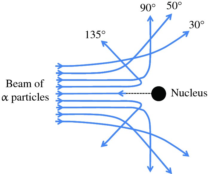
Figure 2.2 The scattering of α particles by a gold nucleus. The scattering angle increases as the α particles approach closer to the nucleus, and these particles can be scattered through very large angles, up to 180°.
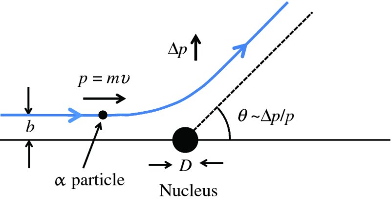
Figure 2.3 The deflection angle, θ, that an α particle experiences as it passes close to a gold nucleus. The distance b is called the impact parameter. The deflection angle is given by the ratio Δp/p, where p is the momentum of the incident α particle and Δp is the sideways momentum that results from the electrostatic repulsion.
where ϵ0 is the permittivity of free space. The deflection angle θ is given by the ratio Δp/p, where p is the momentum of the incident α particle and Δp is the sideways momentum that results from the electrostatic interaction. Hence we have
where m is the mass of the α particle and
 is its kinetic energy. We see that the deflection angle is inversely proportional
to nuclear size D. For gold (Z = 79) and for an α particle with an energy of 5 MeV, we obtain
is its kinetic energy. We see that the deflection angle is inversely proportional
to nuclear size D. For gold (Z = 79) and for an α particle with an energy of 5 MeV, we obtain
For a large angle of deflection, D must be ∼10− 14 m.
Rutherford made a detailed analysis of the angular distribution to be expected for
α particles that are deflected through large angles from a positively charged nucleus
of small dimension. He assumed that the α particle does not penetrate the nuclear
region so that the α particle and the nucleus act like point charges as far as the
electrostatic force is concerned. He also assumed that the mass of the nucleus is
so much greater than the mass of the α particle that the nucleus remains fixed in
space during the scattering process. His analysis was based on a classical treatment
of the electrostatic force between charged particles under the conservation of energy
and angular momentum about the target nucleus. This analysis leads to an expression
for
 , which is the number of detected α particles detected per unit area on the flourescent screen at a deflection angle θ:
where I is the number of incident α particles, n is the number of nuclei per unit volume, t is the thickness of the foil and r is the distance of the screen from the foil.2 This expression predicts how
 depends on the deflection angle θ, the atomic number Z of the atoms in the foil, and the kinetic energy E of the incident α particles. The critical features are the inverse-square dependence
on E and the strong dependence on θ. The dependence of
depends on the deflection angle θ, the atomic number Z of the atoms in the foil, and the kinetic energy E of the incident α particles. The critical features are the inverse-square dependence
on E and the strong dependence on θ. The dependence of
 on θ is shown in Figure 2.4, where the logarithmic scale of the vertical axis may be noted. Even though the number
of detected particles is predicted to fall very sharply with increasing θ, the number at large angles remains appreciable, unlike the predictions of rival
theories. Geiger and Marsden confirmed the predictions of Rutherford's expression
for heavy nuclei like gold and, in particular, the angular behaviour of the scattered
α particles, and consequently the Rutherford model of the atom was adopted. By comparing
the observed angular behaviour of the α particles with the predictions of his expression,
Rutherford was able to obtain a better value for the nuclear radius, which he found
to be approximately 10 fm.
on θ is shown in Figure 2.4, where the logarithmic scale of the vertical axis may be noted. Even though the number
of detected particles is predicted to fall very sharply with increasing θ, the number at large angles remains appreciable, unlike the predictions of rival
theories. Geiger and Marsden confirmed the predictions of Rutherford's expression
for heavy nuclei like gold and, in particular, the angular behaviour of the scattered
α particles, and consequently the Rutherford model of the atom was adopted. By comparing
the observed angular behaviour of the α particles with the predictions of his expression,
Rutherford was able to obtain a better value for the nuclear radius, which he found
to be approximately 10 fm.
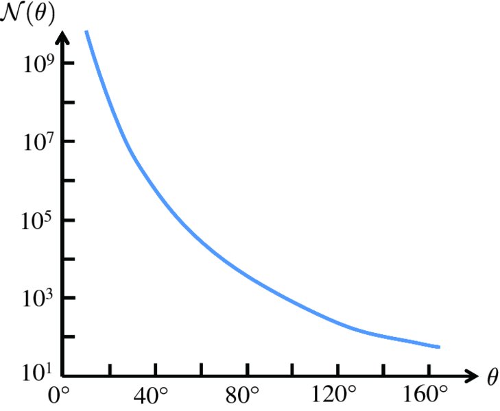
Figure 2.4 The [sin 4(θ/2)]− 1angular dependence of
 , the number of α particles detected per unit area on the fluorescent screen. Note
the logarithmic scale for
, the number of α particles detected per unit area on the fluorescent screen. Note
the logarithmic scale for
 . Although
 falls rapidly with increasing scattering angle θ, a significant number of α particles are detected at very large angles.
Rutherford was fortunate in two ways. The scattering of an α particle by a nucleus is properly described by quantum mechanics. However, for this particular case, the quantum mechanical treatment of the scattering process gives exactly the same result as the classical treatment. Moreover, a 5 MeV α particle does not have enough kinetic energy to penetrate the nucleus of a high-Z nuclide like gold and so Rutherford's assumption of two point charges repelled by electrostatic repulsion was valid.
Experiments using foils of metals with low Z, like aluminium, were also investigated. For these light metals, it was found that Rutherford's expression no longer fitted the experimental data at large angles. This is because the electrostatic repulsion between the α particle and the low-Z nucleus is reduced to the extent that the α particles could penetrate the nucleus at their distances of closest approach. In this case, the nucleus and the α particles can no longer be treated as point charges. Moreover, the α particle comes under the influence of the nuclear force, which operates within the nucleus. This divergence from Rutherford's expression can also be observed by detecting the number of α particles scattered through a particular angle, say 60°, and varying the energy of the incident α particle. The results of such an experiment using a lead foil are shown in Figure 2.5. At lower energies of the α particles, the scattering data are in agreement with the predictions of Rutherford's expression, indicated by the blue curve. However, when the energy of the incident α particle is increased to the point where it can penetrate the nucleus, Rutherford's model breaks down. The α particle and the nucleus can no longer be treated as point charges and the α particle comes under the influence of the nuclear force. All models of physical systems have limitations. However, seeing under what circumstances they break down usually leads to new physical insight.
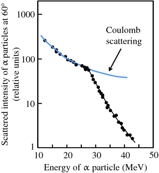
Figure 2.5 Experimental data for the scattering of α particles through a fixed angle of 60° by a lead target shows the breakdown of the Rutherford scattering formula. At an α-particle energy of about 27.5 eV, the data abruptly depart from scattering due to purely electrostatic repulsion. Above this energy the α particles get close enough to the nucleus to come under the influence of the strong but short-range nuclear force.
2.1.3 The distributions of nuclear matter and charge
Since Rutherford's first scattering experiments, atomic nuclei have been extensively investigated by firing high-energy particles at them. In addition to α particles, these experiments have used neutrons and electrons. Electrons are not affected by the nuclear force that exists between protons and neutrons and so they probe the distribution of nuclear charge. By contrast, neutrons have no charge, but interact with protons and other neutrons through the nuclear force and so they probe the distribution of nuclear matter.
From quantum mechanics we know that particles have a wave-like character. This was demonstrated by Clinton Davisson and Lester Germer in 1927. They fired a beam of electrons at the surface of a metal, which happened to be a well-crystallised piece of nickel. They found that the electrons were diffracted by the crystal structure, just as a beam of X-rays is diffracted by a crystal. Any particle with momentum p has an associated wavelength λ that is given by the de Broglie relationship:

where h is Planck's constant. If we want to ‘see’ an object, we need to use radiation that has a wavelength that is smaller, or at least of the same size, as the dimensions of the object. For example, the electrons in an electron microscope have a de Broglie wavelength that is ∼105 times smaller than the wavelength of visible light. Consequently, they are used to see objects that are too small to be seen with a conventional microscope. So it is with nuclei; the de Broglie wavelength of the incident probe particles must be small compared with the nuclear dimensions. We have seen that nuclear diameters are ∼10 fm, and so we require the de Broglie wavelength of the incident particles to be less than about this value. This means that neutrons must have an energy that is greater than about 2 MeV, while electrons must have an energy greater than about 100 MeV. This is a relativistic energy for an electron because its rest mass is 0.51 MeV.
The typical form of the charge distribution of a nucleus, obtained from electron scattering experiments, is illustrated schematically in Figure 2.6. In this figure, the charge density, ρ(r), is plotted as a function of radial distance, r, from the centre of the nucleus. The charge distribution can be characterised by two parameters: the mean radius R, where the density is half its central value and the skin thickness over which ρ(r) drops from 90% to 10% of its maximum value. When a range of nuclides was investigated, it was found that
- the nuclear charge density is roughly constant in the central region of a nuclide and is nearly the same for all nuclides;
- the mean nuclear radius R steadily increases with mass number A according to:
(2.6)
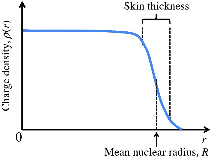
Figure 2.6 Typical form of the distribution of charge density, ρ(r), for a nucleus as a function of radial distance, r, from the centre of the nucleus. R represents the mean nuclear radius. The skin thickness is the distance over which ρ(r) falls from 90% to 10% of its maximum value. The charge density is roughly uniform over the central region of a nucleus.
where R0 is a constant equal to 1.2 fm.
Complimentary experiments using neutron scattering show that the mass distribution of a nucleus is very similar to its charge distribution; the radii of nuclides deduced from charge and mass distributions give values that are the same within about 0.1 fm. The physical explanation of this consistency between mass and charge distributions is that the combination of nuclear and electrostatic forces results in a roughly constant mix of protons and neutrons in the nucleus. That nuclear matter has a constant ‘density’ is consistent with the nuclear radius being proportional to A1/3, as its volume is then proportional to A and its mass is also proportional to A. It also follows that the number of nucleons per unit volume is roughly constant, which, as we shall see, gives valuable physical insights into the nature of the nuclear force. Experimental measurements show that the density of nuclear matter is ∼2 × 10¹⁷ kg/m3, which is 2 × 10¹⁴ times larger than the density of water.
In contrast to nuclei, where nuclear radius steadily increases with mass number, all atoms have roughly the same size. This constancy in atomic radius arises because, as the number of electrons in an atom increases, so also does the number of protons in the nucleus. This increases the nuclear charge, and the attractive electrostatic force acting on the electrons correspondingly increases.
2.1.4 The mass of a nucleus
A good deal of valuable information can be obtained about nuclei from the accurate determination of their masses, as we shall see. However, it is in general very difficult to measure the mass of a bare nucleus, because we would have to strip away all the atomic electrons. Instead we measure the mass of the atom and deduce the nuclear mass from the atomic mass. Or rather, we measure the mass of the atomic ion where just one electron has been removed; it is straightforward to account for the mass of the missing electron. The mass of the atomic ion is measured by exploiting its behaviour in electric and magnetic fields using the technique of mass spectroscopy.
A schematic diagram of a conventional mass spectrometer is shown in Figure 2.7. It consists of an atomic ion source, a velocity selector, a momentum selector to separate the atomic ions according to their mass and an ion detector. The ion source may consist of a vapour of the atom of interest, which is bombarded with an electron beam, and this ionises the atoms. Alternatively, it may be a discharge tube in which the electrodes are coated with the atoms of interest. Either way, the ions are produced with a broad range of thermal energies and consequently they have a broad range of kinetic energies. This would smear out any peaks in the mass spectrum so that individual mass peaks could not be resolved. The purpose of the velocity selector is to filter the ions according to their kinetic energy so that the ion beam emerging from the selector has a very narrow spread of velocities. In the velocity selector there is a pair of parallel electrostatic plates that have opposite polarity. These produce an electric field E that is perpendicular to the direction of the ion beam. These plates are immersed in a magnetic field B1 whose direction is perpendicular to the electric field direction and also to the ion beam direction. The electric and magnetic fields act in opposite directions and ions pass through the selector for which qE = qvB1, where q is the charge of the ion and v is its velocity, which is therefore given by

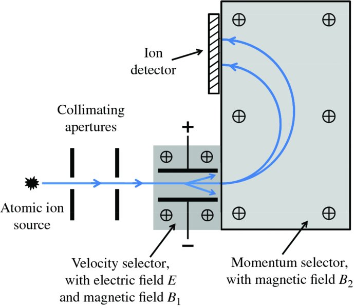
Figure 2.7 Schematic diagram of a mass spectrometer. The collimating apertures define a narrow beam of ions from the source. The velocity selector filters the ions according to their velocity and the velocity-selected ions are injected into the momentum selector. The momentum selector disperses the ions according to their mass and a mass spectrum is recorded on the ion detector. The velocity and momentum selectors are immersed in magnetic fields B1 and B2, respectively, as indicated by the ⊗ symbols. In the velocity selector there is also an electric field E that is perpendicular to the magnetic field B1.
The velocity-selected ions are then injected into the momentum selector, which has a magnetic field B2 that is again perpendicular to the ion beam direction. The ions pass through this magnetic field and follow a circular path according to
where M is the mass of the ion. The radius r depends on the ion momentum, i.e.

Usually the magnetic fields of the velocity and momentum selectors are the same, i.e. B1 = B2 = B, and, substituting for v from Equation (2.7), we obtain
Ions of different mass have different values of r and are dispersed across the detector as illustrated in Figure 2.7. By analogy, a glass prism disperses white light according to wavelength. The ion detector was traditionally a photographic plate, but now an electronic detector is used. Note that r is directly proportional to M, which means that the mass scale of the spectrometer is linear. Figure 2.8 illustrates a mass spectrum of chlorine, showing the peaks of the two isotopes 35Cl and 37Cl. The relative abundances of these two isotopes are 76% and 24%, respectively, which can be deduced from the relative areas of the peaks in the spectrum.
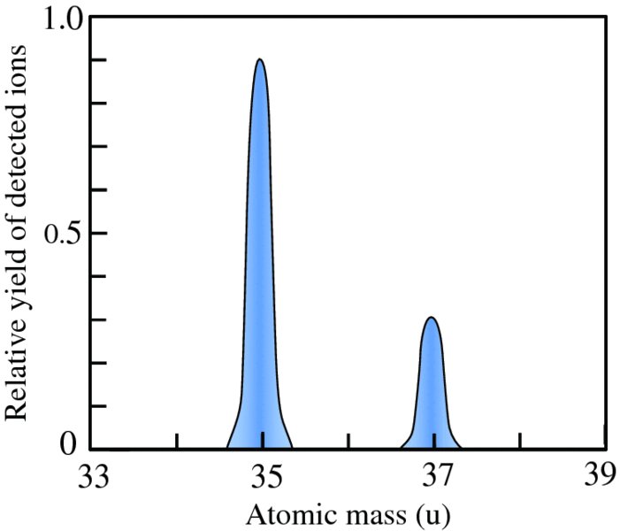
Figure 2.8 A mass spectrum of a naturally occurring sample of chlorine. The relative areas of the peaks due to the 35Cl and 37Cl ions are in the ratio 3:1, reflecting the natural abundances of the two isotopes.
The standard unit of mass for nuclear and atomic physics is the atomic mass unit (u), which is defined such that the mass of a 12C atom is exactly 12 u. In terms of the kg:

Using Einstein's equation E = mc2, we can also express mass in MeV/c2, where
When we discuss the production of energy from nuclear reactions, we will see that it is mass difference that determines the amount of energy that is produced through the equivalence of mass and energy, E = mc2, Equation (2.1). An important aspect of mass spectroscopy is that it can determine the masses of the initial nuclei taking part in a nuclear reaction and those of the product nuclei. From their mass difference, the energy produced in the reaction can be predicted. This requires the masses to be determined to ∼1 part in 107 or 108. To achieve this accuracy, the spectrometer is usually calibrated for one particular atomic mass and other masses are measured with respect to the known mass. This is because it is much easier to measure a mass difference with high precision than the absolute value of the mass from absolute measurements of quantities on the right-hand side of Equation (2.10). The mass difference is deduced from the separation of the two mass peaks on the ion detector, one due to the calibration mass and the other due to the unknown mass.
New experimental techniques have made it possible to confine atomic ions in traps consisting of combined electrostatic and magnetic fields. The ions oscillate in these fields and can be contained in the trap for extended periods of time, rather like a chemical sample in a test tube. By measuring the cyclotron frequency of the ion in the magnetic field, the mass of the ion can be determined. As this is a measurement of frequency, the accuracy is extremely high: ∼1 part in 1011 for stable nuclides.
2.1.5 The charge of a nucleus
The determination of nuclear charge was first achieved by Henry Moseley in 1913. He did this by observing the effects of the nuclear charge on atomic energy levels. In particular, he studied in detail the X-ray spectra of the atoms. These spectra contain sharp peaks called characteristic X-rays that occur at different wavelengths for different elements. Moseley measured the wavelengths of these characteristic X-rays by diffracting them with a crystal. Fortunately, the technique of crystal diffraction had just been developed by W.L. Bragg and his father W.H. Bragg. Moseley found that the wavelengths and frequencies of the characteristic X-ray lines vary smoothly from one element to the next. Furthermore, he found that the measured frequencies of the most intense line in the spectra, known as the Kα line, could be fitted within experimental accuracy by the empirical formula
where ν is the X-ray frequency, Z is the nuclear charge and C is a constant with the value 2.48 × 10¹⁵ Hz. Equation (2.13) is called Moseley's law. It gives a linear relationship between the square root of the frequency
 and (Z − 1), which is illustrated in Figure 2.9. This graph has an intercept at Z = 1, confirming Moseley's law. To find the value of Z for an element we simply measure the frequency of its Kα characteristic line and insert its value into Equation (2.13).
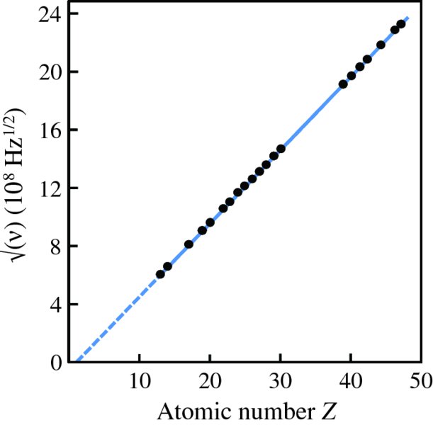
Figure 2.9 A plot of the square root of the frequency ν of the Kα characteristic X-ray line of an atom versus its atomic number Z. The linear dependence of
 on Z is in agreement with Moseley's law.
It is important to understand the physics behind the results of any experiment. Moseley interpreted his results using an extension of the Bohr model of the atom, which was published in the same year. In Bohr's model of the hydrogen atom, the single electron can exist in orbitals around the proton nucleus that have well defined energies. Bohr obtained the following expression for the energy En of the nth orbital:
where m, e, ϵ0 and h are fundamental constants, Z is the charge on the nucleus and n is called the principal quantum number of the orbital. n can take on values 1, 2, 3, … (Z = 1 for hydrogen, but we will retain the symbol Z for reasons that will soon become apparent). The minus sign indicates that the electron is bound to the proton, where En gives the binding energy; energy En is required to eject the electron from the nth orbital. Inserting the values of the fundamental constants, we find
When an electron makes a transition from initial orbital ni to lower-lying orbital nf, energy is released in the form of a photon whose energy Eph is Ei − Ef, which is given by
For example, when an electron in the n = 4 orbital of hydrogen falls to the n = 3 orbital, a photon is released with an energy of 1.89 eV. This corresponds to a wavelength that is given by λ = hc/E, and which is equal to 564 nm. This lies in the visible region of the electromagnetic spectrum.
In multi-electron atoms, the electrons exist in shells that surround the nucleus. Again these shells are characterised by their principal quantum number n. Roughly speaking, electrons in the same shell are at about the same distance from the nucleus. X-rays correspond to transitions between the inner shells of an atom. They are produced, for example, when a metal target such as copper is bombarded with a beam of very energetic (∼10–100 keV) electrons. An incident electron may knock out an electron from the innermost shell of the target atom, with n = 1, as shown in Figure 2.10(a). The ejected electron leaves behind a vacancy or hole in that shell. This vacancy may then be filled by an atomic electron from another shell, say the n = 2 shell, as shown in Figure 2.10(b). This is accompanied by the emission of an X-ray, whose energy is equal to the energy difference between the energies of initial (n = 2) and final (n = 1) shells of the atom. These transitions are exactly analogous to those between the outer shells of atoms. However, the inner-shell electrons are much closer to the nucleus and, consequently, are much more tightly bound. As a result, the energy differences between the inner shells are correspondingly large and the X-rays have short wavelengths, ∼0.1 nm.
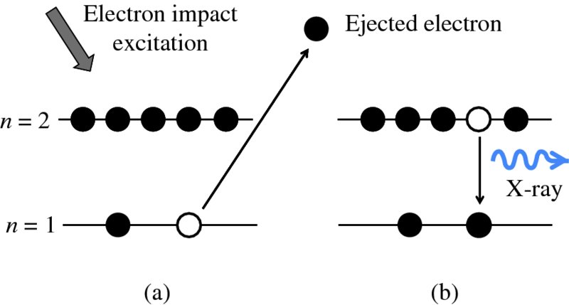
Figure 2.10 The process of X-ray emission from an atom. (a) An incident electron knocks out an atomic electron from the n = 1 shell, leaving a vacancy in that shell. (b) The resulting vacancy in the n = 1 shell is filled by an atomic electron from the n = 2 shell and this is accompanied by the emission of an X-ray.
The n = 1 shell of an atom contains two electrons, and when one is knocked out of the shell one electron remains. Thus an electron that falls from the n = 2 shell into the vacancy in the n = 1 shell sees an effective nuclear charge, Zeff, equal to + (Z − 1)e, due to the Z protons in the nucleus and the remaining electron in the n = 1 shell; the n = 1 electron screens the n = 2 electron from the nucleus. Moseley modified the Bohr model to take account of the effective nuclear charge that an electron experiences. In terms of Moseley's modified formula, we write the energy level En of an atom as
The energy of a resulting X-ray is then
Taking Zeff = (Z − 1) with ni and nf equal to 2 and 1, respectively, we obtain

The frequency, ν, of the emitted X-ray is then
The form of this equation is in agreement with Moseley's Equation (2.15). Moreover, the value of the constant in Equation (2.20) is in good agreement with the value of the constant C obtained by Moseley.
Moseley's work provided for the first time a way to determine the atomic number Z of an element. As a result, the correct sequence of elements in the periodic table could be established. Previously the ordering had been in terms of their atomic mass, which had led to some inaccurate ordering. In addition, Moseley found gaps that indicated the existence of elements that were not known at the time. These elements were subsequently discovered, some many years later.
2.1.6 Nuclear binding energy
The neutrons and protons in a nucleus are held together by strong attractive forces, as we will describe in Section 2.2. Therefore, work must be done to separate these nucleons from each other until they are a large distance apart, i.e. energy must be supplied to the nucleus to separate it into its individual nucleons. The energy that must be added to a nucleus to separate it into its individual neutrons and protons is called the binding energy, B, of the nucleus. Binding energy is not an energy that resides in a nucleus, like kinetic energy. Rather, it is the energy equivalent of mass through Einstein's mass–energy relationship

We thus expect the mass of the nucleus to be less than the sum of the masses of the constituent nucleons, and this is indeed the case. The difference between the mass of the nucleus and the constituent nucleons is called the mass defect Δm. In terms of the mass defect, the binding energy is equal to Δmc2.
We recall that it is atomic masses that are measured in mass spectroscopy. If the mass of an atom is AZM, the mass of its nucleus is (AZM − Zme), where me is the mass of the electron. Hence, the mass difference, Δm, between a nucleus and its constituent nucleons is

where mp and mn are the masses of the proton and the neutron, respectively. But (mp + me) is just the mass of a neutral hydrogen atom. Hence, we have
and finally, the binding energy B of the nucleus is given by

where MH is the mass of the neutral hydrogen atom.
The more tightly bound the nucleons are in a nucleus, the more energy it takes to separate them. For a given value of A ( = Z + N), there may be different combinations of Z and N. The combination that gives the largest total binding energy will be the most stable nuclide. It follows from Equation (2.23) that the most stable nuclide will also be the one with the lowest mass, AZM.
The electrons in an atom also have binding energy. For example, the electron in the ground state of hydrogen has a binding energy of 13.6 eV, i.e. this amount of energy must be added to the atom to remove the electron. We are able to neglect the binding energies of the atomic electrons when deducing the binding energy of a nucleus for two main reasons. First, electron binding energies are negligible compared with the rest-mass energies that appear in Equation (2.23). For example, an atom with an atomic number A of, say, 100 has a rest mass energy of ∼1011 eV, while the most tightly bound electrons, those in the inner shells of an atom, have energies of ∼104 eV. Secondly, electronic binding energies tend to cancel out in calculations of differences in nuclear binding energy between two different nuclides.
As an example of nuclear binding energy, we consider deuterium 21D, which is an isotope of hydrogen, with Z = 1. The deuterium nucleus contains a single neutron and a single proton. From precise mass spectroscopic measurements we know that the masses of deuterium and hydrogen atoms are, respectively, 2.014 102 and 1.007 825 u, while the mass of the neutron is 1.008 665 u. Hence, the mass defect is

and the binding energy B is
We have given all the steps of this calculation for the sake of clarity. However, we note that it is more convenient to use the conversion factor
so using Equation (2.23) directly, we have

We can also determine the binding energy by bringing a proton (1H) and a neutron together to form deuterium and measuring the energy that is emitted in the reaction, which is in the form of a γ-ray:
The observed energy of the γ-ray, less a small correction due to the recoil energy, is found to be 2.225 MeV in close agreement with the value deduced from the mass spectroscopic measurements. Alternatively, we can have the reverse reaction called photo-dissociation, in which we split deuterium into a proton (1H) and a neutron by the absorption of a γ-ray:
as illustrated schematically in Figure 2.11. The minimum energy that the γ-ray must have to do this is equal to the binding energy, again corrected for the recoil of the final products. The measured value for the minimum energy is 2.224 MeV, again in close agreement with the value deduced from the mass spectroscopic measurements.
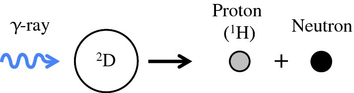
Figure 2.11 The disintegration of a deuterium nucleus into a proton (1H) and a neutron by the absorption of a γ-ray.
2.1.7 Binding energy curve of the nuclides
We could repeat the exercise of the previous section to deduce the nuclear binding energy B for all the elements in the periodic table from their accurately measured atomic mass. The deduced values of B could then be plotted versus atomic mass number A. However, we obtain more physical insight into the nature of the nucleus by plotting B/A versus A, where B/A is the binding energy per nucleon. The resulting curve is presented in Figure 2.12 for the stable nuclides. Several features of this curve are immediately apparent:
- The binding energy per nucleon is roughly constant at ∼8 MeV except for nuclides lighter than 12C. The relative flatness of the curve shows that B is approximately proportional to A. This is a very significant feature as it indicates that each nucleon in the nucleus is attracted only to its nearest neighbours. If each nucleon attracted all the other (A − 1) nucleons, there would be a total of A(A − 1) bonds and B would instead be proportional to A(A − 1) ∼ A2, not to A. In turn, this demonstrates that the nuclear force must operate over a very short range. This is analogous to the molecules in a drop of water, where the molecules interact only with their nearest neighbours.
- The curve has a broad maximum at A ∼ 60. This feature is of great physical and practical importance. It indicates that we can release energy by splitting a heavy nucleus into two less massive and more tightly bound nuclei that lie closer to the maximum in the curve (nuclear fission). Alternatively, we can release energy by fusing two light nuclei together to produce a more tightly bound nucleus, which again lies closer to the curve maximum (nuclear fusion).
- The curve gradually reduces in height at high A. This is due to the electrostatic repulsion of the protons. In contrast to the short-range nuclear attractive force, the electrostatic force is long range, falling as 1/r2, where r is the proton–proton separation. Consequently, each proton repels all the other protons. This repulsion reduces the binding energy. Eventually, for very large A, the electrostatic repulsion dominates the nuclear attraction and nuclides with A greater than about 210 are unstable and radioactively decay.
- There is a pronounced spike in the curve at A = 4. This shows that the binding energy of the helium nucleus, i.e. the α particle, is particularly large. There are also peaks, although less pronounced, at A = 12 and 16. These spikes are an indication that neutrons and protons are arranged in shells, just as the electrons in an atom are arranged in shells. These more tightly bound nuclides have closed shells of nucleons. This is again analogous to the situation for atoms that have closed electronic shells like the rare gases, which have relatively high ionisation energies.
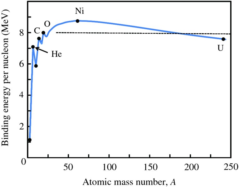
Figure 2.12 A plot of binding energy per nucleon B/A versus atomic mass number A for the stable nuclides. Except for the region of low mass number, the binding energy curve has a roughly constant value of ∼8 MeV, indicating that the total binding energy of a nuclide is approximately proportional to A. Peaks occur at 4He, 12C and 16O, as these nuclides have particularly high values of binding energy. Also indicated are the nuclides Ni (nickel), which occurs close to the maximum of the curve, and U (uranium), which occurs at the high end of the atomic mass range.
2.1.8 The semi-empirical mass formula
There are some similarities between nucleons in a nucleus and molecules in a drop of water, as we have already hinted. In particular, the density of water is constant and independent of the size of the water drop. Moreover, the amount of energy it takes to vapourise a drop of water is directly proportional to the volume of the drop, i.e. the amount of energy required per molecule is constant. Similarly, the density of nuclear matter is approximately the same for all nuclides and the binding energy per nucleon is fairly constant, except for the lightest nuclides. These considerations led to the liquid drop model of the nucleus, where individual nucleons are considered to be analogues of molecules in a liquid, held together by short-range interactions and surface tension effects. Molecules are held together by covalent bonding, which operates over a short range so that molecules bind only to their nearest neighbours, just as nucleons bind only to their nearest neighbours. We have also hinted at indications that nuclei have a shell-like structure where the nucleons occupy shells, just as electrons occupy shells in atoms. Such indications lead to the shell model of the nucleus. In this model, each nucleon moves independently with an average potential energy due to the nuclear force of all the other nucleons and the electrostatic force of the other protons (see also Section 2.2.3).
Based upon these considerations, we can attempt to derive a formula for the binding energy B(Z, A) of a nuclide in terms of its Z and A values. This formula has the following five contributions.
Volume term
The value of B/A is fairly constant in the binding energy curve across most of the range of the stable nuclides, i.e. B depends roughly linearly on A. Hence, the most obvious, and also the most important, term in a formula for B(Z, A) is a term avolA that depends linearly on A and where avol is a constant. As the volume of a nucleus is approximately proportional to A, this term is called the volume term.
Surface term
The nucleons at the surface of a nucleus are less tightly bound than those in the interior because they have no neighbours outside the surface. This leads to a decrease in binding energy. As the radius of a nucleus is proportional to A1/3, the surface area is proportional to A2/3. This results in the surface term − asurfA2/3, where asurf is a constant and the minus sign indicates that this term reduces the binding energy. This surface tension effect helps to explain why nucleii are nearly spherical in shape, the shape that water droplets seek to attain.
Coulomb term
This term arises from the electrostatic repulsion of the protons that tends to make the nucleus less tightly bound. Electrostatic repulsion is a long-range force and so each proton interacts with all the other (Z − 1) protons. As there are Z protons, the total repulsive Coulomb energy is proportional to Z(Z − 1) ∼ Z2. The Coulomb energy also depends on the inverse of the radius of the nucleus. We thus obtain the Coulomb term − aCoulZ2/A1/3, where aCoul is a constant and, again, the minus sign indicates that this term reduces the binding energy. [We can compare this result with the electrical potential energy of a uniformly charged sphere of radius R and total charge Q, which is equal to 3/5(Q2/4πϵ0R).]
(These first three terms would also arise for the case of a charged liquid drop in accordance with the liquid drop model of the nucleus. The following two terms are accounted for in terms of the way in which nucleons occupy the shell-like structure of a nucleus.)
Asymmetry term
The chart of stable nuclides shows that there is a preference for light nuclei to have Z ≈ N, i.e. Z ≈ A/2, (see also Section 2.3.1), although this tendency is reduced when A is large and electrostatic repulsion of the protons increases. A suitable term in B(Z, A) to take this into account is − asym(A − 2Z)2/A and is called the asymmetry term, where asym is a constant. This term is zero when Z = A/2 but when Z ≠ A/2, it appears as a negative term, reducing the binding energy. Also, the asymmetry term reduces in importance as A increases.
Pairing term
The nuclear force favours pairing of like nucleons; the nuclide is more tightly bound if both Z and N are even, but less tightly bound if both Z and N are odd. This is accounted for by a pairing term δ in B(Z, A). δ is positive if Z and N are both even, negative if both Z and N are odd, and zero if either Z or N is odd (A odd). δ can be expressed as apairA− 3/4.
Combining the five terms, we obtain the formula B(Z, A) for the binding energy of a nuclide:

In Section 2.1.6. we saw that we could deduce the binding energy, B, of a nuclide from a knowledge of its atomic mass, AZM:
When we substitute B(Z, A) from Equation (2.27) into Equation (2.23), we obtain

This is the semi-empirical mass formula. It enables accurate values of an atomic mass to be predicted and it applies to both stable and, very usefully, unstable nuclides. This makes it of great practical importance because it can predict, for example, the mass difference in a particular nuclear reaction and hence the amount of energy that can be obtained from that reaction. The formula is described as semi-empirical because it is based on both experimental observations and theoretical considerations.
By dividing Equation (2.27) by mass number A, we obtain a formula for B(Z, A)/A, the binding energy per nucleon. Furthermore, we can fit the resulting formula to the binding energy curve in Figure 2.12, by adjusting the values of the constants avol, asurf, aCoul, asym, and apair to give the best agreement between B(Z, A)/A and the binding energy curve. One set of values is:

2.2 Nuclear forces and energies
2.2.1 Characteristics of the nuclear force
The neutrons and protons in a nucleus are bound together by the so-called nuclear force. This force is understood to be a secondary effect of the strong force that binds quarks together to form the neutrons and protons themselves. This more powerful strong force is mediated by particles called gluons, which act to hold quarks together. Quarks, gluons and their dynamics are mostly confined within nucleons, but residual influences extend slightly beyond nucleon boundaries to give rise to the nuclear force. (The strong force is considered to be one of the four fundamental forces of nature, the others being the gravitational force, the electromagnetic force and the weak nuclear force, which we will meet when we discuss β decay.) The nuclear force that binds the neutrons and protons together has the following properties:
- It has a strongly attractive component, which acts only over a very small range, ∼ few fm.
- It has a repulsive component at very short distances, less than ∼0.5 fm, which keeps the nucleons apart.
- Within its range of operation, the nuclear force is much stronger than the electrostatic force. For example, the nuclear force acting between two protons at a separation of 2 fm is about 100 times stronger than the electrostatic force. Consequently, the nuclear force can overcome the electrostatic repulsion of the protons in the nucleus.
- It is charge-independent, i.e. the nuclear force between protons is the same as the nuclear force between neutrons and the same as the nuclear force between protons and neutrons.
- There is no nuclear force between electrons and either protons or neutrons.
- The nuclear force favours pairing of protons and of neutrons with opposite spins. Hence the α particle with two protons and two neutrons is an exceptionally stable nucleus, as we have already seen.
The nuclear force between two nucleons results in a potential energy curve of the form illustrated in Figure 2.13, which shows the potential energy as a function of the separation of the two nucleons. The curve applies to the case of two neutrons or a proton and a neutron, for which there is no electrostatic repulsion. At large separation, the potential energy is zero. As the two nucleons approach each other, at around a few fm, they experience the strongly attractive nuclear force that leads to a decrease in potential energy. At short distances, below about 0.5 fm, the nuclear force becomes repulsive and the potential energy increases sharply. A minimum in the potential energy occurs at a separation where the attractive and repulsive forces are equal and opposite. This is a position of equilibrium and so the two nucleons tend to maintain this separation.
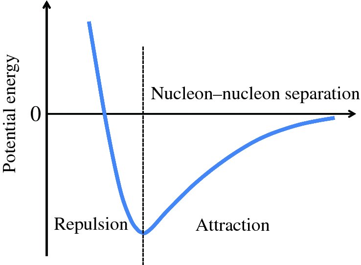
Figure 2.13 The potential energy of two nucleons as a function of their separation, resulting from the strong nuclear force between them. A minimum in the potential energy occurs at an equilibrium separation where the repulsive component of the nuclear force is balanced by the attractive component.
2.2.2 Nuclear energies
Figure 2.13 illustrates the potential energy between two nucleons as a function of their separation. We now consider the energies of nucleons that exist within a nucleus. We saw above that there is an equilibrium separation between nucleons and so the nucleons within a nucleus tend to maintain an average separation with respect to their neighbours. Furthermore, as the nuclear force has a very short range, nucleons interact only with their nearest neighbours. Consequently, a nucleon has an approximately constant energy due to the attraction of its neighbours. We can consider the nucleons in a nucleus as particles that exist within a potential well. Such a potential well for the neutrons in the nucleus is shown in Figure 2.14(a). In this figure, the horizontal axis represents the radial distance, r, from the centre of the nucleus and the vertical axis represents the potential energy, V(r), of the neutrons. The bottom of the well is flat as the neutrons have an approximately constant energy of attraction and so their potential energy is approximately constant in the nuclear interior. Because the neutrons are bound to the nucleus, the bottom of the well lies below the zero of potential energy. The well does not have sharp sides because the nuclear force does not fall off abruptly and also because the distribution of neutrons near the surface does not fall off abruptly (see Figure 2.6). The width of the well is essentially the nuclear radius. The depth of the well depends on the number of nucleons in the nucleus but is ∼50 MeV. When it is away from the nucleus, a neutron does not experience any force and its potential energy is zero. If it approaches the nuclear surface, it experiences the attractive nuclear force and ‘falls’ into the nuclear interior with a gain in kinetic energy corresponding to a decrease in its potential energy.
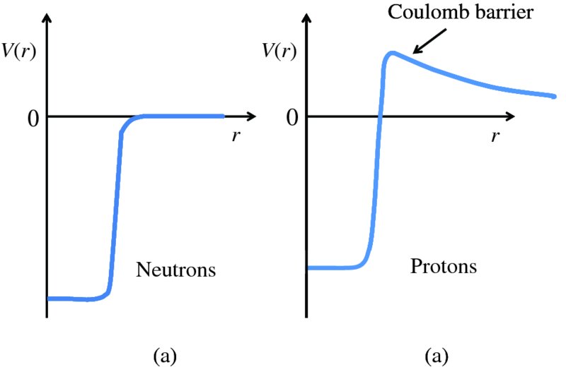
Figure 2.14 (a) The potential energy function, V(r), for neutrons that are bound in a nucleus, where the potential energy V is plotted as function of radial distance r from the centre of the nucleus. In the interior of the nucleus, the potential energy is approximately constant, as depicted by the flat bottom of the potential well. (b) V(r) for protons that are bound in a nucleus, again plotted as function of r. In addition to the nuclear force, protons also experience electrostatic repulsive due to other protons. The addition of this electrostatic repulsion to the nuclear attraction reduces the depth of the potential well for protons. Further away from the nucleus, the protons feel just the long-range electrostatic force, and the combination of the attractive nuclear force and the repulsive electrostatic force results in the formation of a Coulomb barrier.
The protons in a nucleus experience the same nuclear force as the neutrons. Hence, they have a component in their potential energy function due the nuclear force that is the same as for the neutrons. In addition, however, protons also experience the repulsive electrostatic force due to other protons. When we add this electrostatic repulsion to the attraction due to the nuclear force, we get the total potential energy function V(r) for the protons that is shown in Figure 2.14(b). Within the nucleus, the electrostatic repulsion reduces the depth of the potential well. Further away from the nucleus, the protons feel just the long-range electrostatic force. The combination of the attractive nuclear force and the repulsive electrostatic force results in the formation of a potential barrier as shown in Figure 2.14(b). This is called the Coulomb barrier. It plays a crucially important role in maintaining the stability of the Universe, as it prevents low-energy nuclei coming into contact with each other and forming a heavier nucleus, even though that heavier nucleus would be more stable. As the positively charged nuclei approach each other, they are repelled by the long-range electrostatic force before they can come under the influence of the much stronger nuclear force. Indeed, the Coulomb barrier hinders the generation of energy by nuclear fusion, as we will see in Chapter 3. It also plays a role in the mechanism of the radioactive decay of nuclei by α particle emission, as we will discuss in Section 2.3.3.
We can get a rough estimate of the kinetic energy of a nucleon in a nucleus from an important principle of quantum mechanics; namely the uncertainty principle. One statement of this principle is that it is not possible to know the position and the momentum of a particle completely. This is represented by the expression
where Δx is the uncertainty in the particle's position, Δp is the uncertainty in its momentum, and ℏ is h/2π, where h is Planck's constant. It follows that the momentum p of the particle must be at least as large as ℏ/2Δx. Hence, an estimate of the lower limit for the kinetic energy E = p2/2m of a nucleon is given by
Taking a nuclear dimension of 1 fm for Δx we obtain a value for E of ∼5 MeV. When we repeat this exercise for an electron in an atom, and take an atomic dimension of 0.1 nm, we obtain the kinetic energy of the electron to be ∼1 eV, a factor ∼106 smaller. We can begin to see that nuclear reactions will produce much greater amounts of energy than are produced in chemical reactions, which involve atomic electrons. The uncertainty principle also explains why electrons do not reside in the nucleus. Electrons are around 2000 times less massive than nucleons. If an electron were to be confined to a region of dimension ∼1 fm, and taking relativistic effects into account, the electron would have a kinetic energy of ∼100 MeV. This would require a potential barrier of this magnitude to bind the electron and such a barrier does not exist.
When a particle is confined in a potential well, the confinement leads naturally to discrete energy levels that the particle can occupy. This is one of the important results of quantum mechanics, as we describe in Section 2.2.3. It is the basis of the shell model of the nucleus, where we consider that neutrons and protons exist inside nuclei in certain allowed energy levels within a potential well. The situation is analogous to that for atoms, which similarly have discrete energy levels, except that the nuclear energies are the order of a million times larger, as noted earlier. Atomic energy levels are occupied by the atomic electrons. Electrons are spin-1/2 particles and consequently they fill the available atomic energy levels according to the Pauli exclusion principle. This states that no two spin-1/2 particles can have the same set of quantum numbers. Consequently, each energy level can hold only a certain number of electrons; additional electrons have to go into levels that are at higher energy. Neutrons and protons are also spin-1/2 particles and, again, fill the available energy levels of a nucleus according to the Pauli exclusion principle.
We illustrate this arrangement of nucleons in a nucleus with the example of the light nuclide 12C. Because this nuclide has relatively few protons, we can neglect electrostatic repulsion and consider only the potential energy due to the nuclear force. The resulting potential wells are then the same for both neutrons and protons. The potential wells and the first few possible energy levels for 12C are illustrated schematically in Figure 2.15; the separations of the energy levels are not to scale. The potential wells for the neutrons and protons are conventionally drawn back to back as shown. 12C has six protons and six neutrons and these populate the energy levels according to the Pauli exclusion principle, with two nucleons in the lowest energy level and four nucleons in the next level. Protons and neutrons are not identical particles and so the Pauli exclusion principle is not violated when they occupy the same energy levels, as shown.
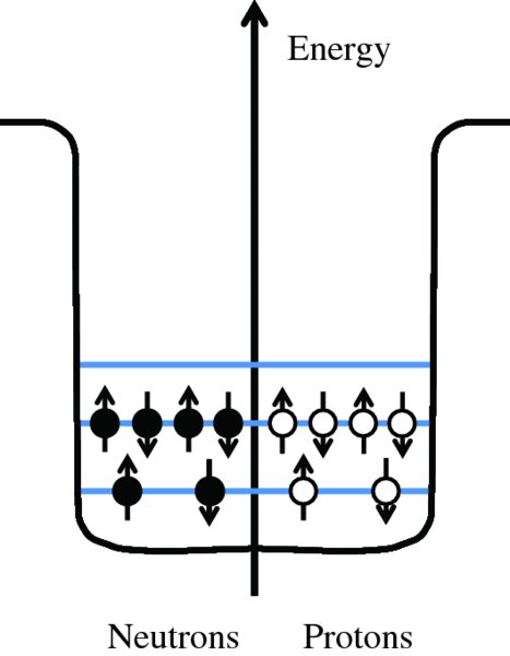
Figure 2.15 Schematic diagram of the first few energy levels in the 12C nucleus, showing the arrangement of the six neutrons and six protons in the levels, which are not drawn to scale. The potential wells for the neutrons and protons are conventionally drawn back to back, as shown. Because 12C has relatively few protons, the electrostatic energy due to proton repulsion can be neglected and only the potential energy due to the nuclear force needs to be considered.
It is found that nuclei with either Z or N = 2, 8, 20, 28, 50, 82 and 126 have a larger value of binding energy per nucleon than predicted by the semi-empirical mass formula. These numbers are the so-called magic numbers. Their existence provides compelling evidence for the shell model of the nucleus, where these values of Z correspond to full shells of nucleons, either neutrons or protons. An analogous situation occurs for atoms. For particular values of Z, corresponding to the rare gases, helium, neon and argon, the ionisation energy of the respective atom is relatively large. Again these atoms have full shells of electrons.
2.2.3 Quantum mechanical description of a particle in a potential well
Calculating the exact potential energy function, V(r), of a nucleus and the resulting energies of the individual nucleons is a formidable task and must be solved with sophisticated methods of quantum mechanics. However, we can gain valuable physical insight into the existence of nuclear energy levels by considering the much simpler case of a particle confined to a one-dimensional potential well. (Indeed, a particle in a one-dimensional well is an important example in quantum mechanics and is applied to many physical situations.) Moreover, we can extend our discussion to see what happens when a particle strikes a potential barrier of finite height; a case that is of importance in α-particle decay.
We are familiar with the case of a taut string that is held between two fixed points. When the string is plucked, standing waves are formed on the string. In particular, only standing waves of particular wavelengths can exist. The condition is nλ/2 = L, where λ is the wavelength, L is the length of the string and n = 1, 2, 3, … (see also Section 4.2.3). Only these values of λ are allowed because of the boundary conditions at the fixed ends. As we have already noted, particles on an atomic or subatomic scale have wave-like properties. Accordingly, the state of such a particle is described by a wave function, just as a disturbance on a taut string is described as a wave. In general the wave function is a function of the three spatial coordinates, x, y and z, and of time t, i.e. ψ(x, y, z, t). The physical meaning of the wave function can be interpreted in the following way. The square of the wave function of a particle at a particular point gives the probability of finding the particle at that point. The particle is most likely to be found where |ψ|2 is large (we write the square of the absolute value of ψ2 as ψ may be a complex quantity). In some cases, the value of ψ is independent of time, in which case the wave function depends only on the spatial coordinates, i.e. ψ = ψ(x, y, z). This occurs, for example, when the particle is in a state of definite energy, which does not change with time. We can determine the wave function of a particle and its associated energy using the Schrödinger equation, named after Erwin Schrödinger who introduced it. The Schrödinger equation plays the role in quantum mechanics that Newton's laws play in classical mechanics. For a particle of mass m and energy E that moves in one dimension along the x-axis, the time-independent Schrödinger equation is
where V(x) is the potential energy and ℏ is as defined earlier. Schrödinger's equation is really a statement that the kinetic energy of the particle [represented by the term − (ℏ2/2m)(d2ψ(x)/dx2)] plus the potential energy [represented by the term V(x)ψ(x)] is equal to the total energy of the particle [represented by the term Eψ(x)], cf. the classical expression:
We can readily apply Schrödinger's equation to the example of a particle in a one-dimensional infinite potential well.
A particle in a one-dimensional infinite potential well
The one-dimensional infinite potential well is shown in Figure 2.16. The potential energy V(x) is zero between x = 0 and x = L, and infinite elsewhere. We consider a particle of mass m and total energy E that can move within the well along the x-axis. As V(x) rises abruptly to infinity at x = 0 and x = L, the particle is confined to the region 0 < x < L and outside this region ψ(x) must be zero, i.e. the particle is confined between two infinitely high rigid walls.
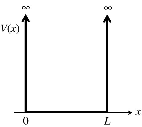
Figure 2.16 The one-dimensional infinite potential well. The potential energy V(x) is zero between x = 0 and x = L, but rises abruptly to infinity at x = 0 and x = L, so that any particle in the well will be confined to the region 0 < x < L.
Between x = 0 and x = L, V(x) = 0 and from Equation (2.30), the wave function must satisfy
The general solution to this equation is

where
As ψ(x) = 0 at x = 0, we have B = 0, giving
As ψ(x) = 0 at x = L, we have

k can have an infinite number of values given by Equation (2.36) and for each value of k there is the corresponding wave function:
[This result is completely analogous to the case of standing waves on a taut string, because the differential equations describing the two situations are of the same form. If in Equation (2.32) we substitute E = p2/2m, with λ = h/p, the de Broglie wavelength of the particle, we obtain
The differential equation describing standing waves on a taut string is
where λ is the wavelength and fn(x) describes the variation of the amplitude A of the wave along the length L of the string. fn(x) has the form fn(x) = Ansin (nπx/L).]
Substituting for
 in Equation (2.35) and substituting the resulting ψn(x) in Equation (2.32), we obtain the possible energy levels En for the particle in the well:
We see that the particle can only have certain discrete values of total energy En, which are given by Equation (2.38). For the infinite potential well there is an infinite number of energy levels, each having its own quantum number n and a corresponding wave function given by Equation (2.35). Figure 2.17(a) shows the wave functions for n = 1, 2, 3, 4 and 5. Again these functions are identical to those for a standing wave on a string. Figure 2.17(b) shows the energy level diagram for the system. The energy levels are quantised and are proportional to n2. We can use Equation (2.38) to make an estimate of the energy of a nucleon in a nucleus. Taking n = 1 and L = 5 fm, and using the known values of the fundamental constants, we obtain E1 ∼ 8 MeV.
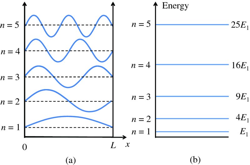
Figure 2.17 (a) The wave functions for a particle confined in an infinite potential well, for quantum number n = 1 to 5. These functions are identical to those for standing waves on a string. (b) The corresponding, quantised energies of the particle in the well, which scale as n2.
A particle in a one-dimensional finite potential well
The potential well confining the nucleons in a nucleus is not infinite in extent (see Figure 2.14), and so we next consider the case of a particle that is bound in a potential well where one of the walls is not infinitely high. This well is illustrated in Figure 2.18 and resembles the form of the potential wells of Figure 2.14. In this case, the potential V(x) is given by
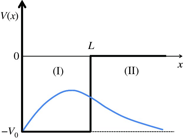
Figure 2.18 A potential well in which one of the walls is not completely rigid; the potential energy does not become infinite at x = L. Also shown is the wave function that corresponds to the ground state of a particle in the well.
When the total energy E of the particle (kinetic energy plus potential energy) is negative, having a value between −V0 and 0, the particle is trapped in the well. The solution of the Schrödinger equation follows the treatment above, but now there are two separate regions, (I) and (II), to consider, as indicated on Figure 2.18, with two separate solutions of the wave equation. As usual, these solutions must comply with the boundary conditions. At x = 0, ψ(x) = 0, as in the previous example. At x = L, both ψ(x) and dψ(x)/dx must be continuous: if ψ(x) or dψ(x)/dx were discontinuous at any point then d2ψ(x)/dx2 would be infinite, which is unphysical.
In region (I); 0 ⩽ x ⩽ L, we have V(x) = −V0, and
Taking into account the boundary condition at x = 0 we obtain the solution
where
 . Again, the wave function has a sinusoidal form.
In region (II), x > L, the potential energy is zero and we have
E is a negative quantity, as the particle is bound and so the solution of Equation (2.41) is

where
 . To ensure that the wave function is finite for x → ∞, B must be zero. Hence, the wave function in region (II) is given by
This quantum mechanical result is dramatically different from the classical result. Classically, the particle is trapped between the walls and cannot exist in the region x > L, as its energy E lies below the top of the wall. Quantum mechanically, however, it can penetrate into the classically forbidden region. This ability to penetrate a classically forbidden region is one of the most important properties of a quantum particle and arises because of its wave nature.
Applying the boundary conditions on ψ(x) and dψ(x)/dx at x = L, we obtain
k1 and k2 are not independent parameters. They are defined by
giving
We thus have two simultaneous equations for k1 and k2. Given the value of V0, these equations can be solved graphically (or numerically) to obtain the values of k1 and k2, and hence the energies of the possible bound states. The form of the ground-state wave function for a particle in the well is shown in Figure 2.18 as the blue curve.
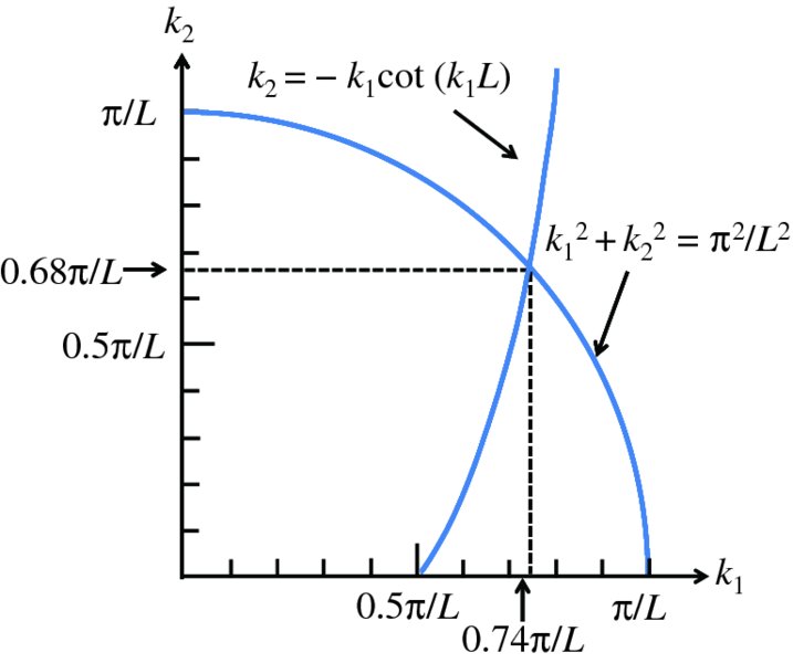
Figure 2.19 Plots of k2 versus k1 to determine the possible energies of a particle in a finite well potential such as that shown in Figure 2.18, with a well depth V0 = ℏ2π2/2mL2. In this case, there is just one bound state.
The deuteron
The proton and the neutron in the deuteron nucleus are bound together by the nuclear force. Because it is a bound system the nucleons move in an attractive potential, representing their mutual attraction, and their total energy must be negative. We can model the deuteron nucleus by a three-dimensional form of the finite potential well. This well is illustrated in Figure 2.20, where the horizontal axis represents the radial distance r. In a similar manner to the one-dimensional case above, we obtain the relation
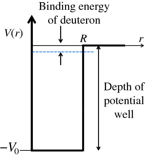
Figure 2.20 A three-dimensional finite potential well to model the deuteron nucleus. This model gives just one bound state of the nucleus with a binding energy of approximately 2 MeV, which is in agreement with the experimentally measured value.
where

and R is taken to be the diameter of the deuteron nucleus. Equation (2.47) is exactly analogous to Equation (2.44). Note that Equations (2.47) and (2.48) connect the depth V0 of the potential well to the diameter R of the nucleus. Knowing the value of R from scattering experiments, we can use the model to predict the value of V0, which is found to be approximately 35 MeV. The model gives just one bound energy level in this potential well, as in the worked example above. Moreover, this level lies just below the top of the well with a binding energy of about 2 MeV, in agreement with the known values of the binding energy that we saw in Section 2.1.6. It is fortunate that deuterium does have a bound state, i.e. that it is a stable nucleus, because deuterium is an essential step in the fusion of nuclei in stars, including our own.
Barrier penetration
The other case that is of interest to us is where a particle is incident upon a potential barrier. In particular, we consider the case where the total energy of the particle E is less than the height of the barrier. This case is illustrated in Figure 2.21, where the particle approaches the barrier from the left. The potential V(x) is given by
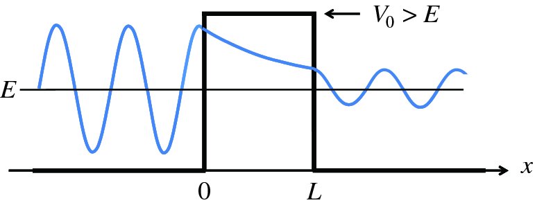
Figure 2.21 A particle of energy E approaches a barrier of height V0, where E < V0. Quantum mechanically, the particle can tunnel through the barrier. The wave function of the particle exhibits an oscillatory behaviour on either side of the barrier and has an exponentially decreasing amplitude within the barrier.
Classically the particle cannot surmount the barrier; it would simply be reflected backwards. However, quantum mechanically the particle has a finite probability of being found to the right of the barrier, i.e. tunnelling through the barrier. We can make an analogy here with barrier penetration by a wave in light optics. If a beam of light is incident upon a glass/air interface at an angle greater than the critical angle, the light beam is completely reflected from the interface. However, there exists a wave disturbance that penetrates a few wavelengths into the air space. If a second block of glass is brought sufficiently close to the glass/air interface, light will pass across the gap into the second glass block, as illustrated in Figure 2.22. The penetration of a particle through a potential barrier is analogous to this because of the wave nature of the particle.
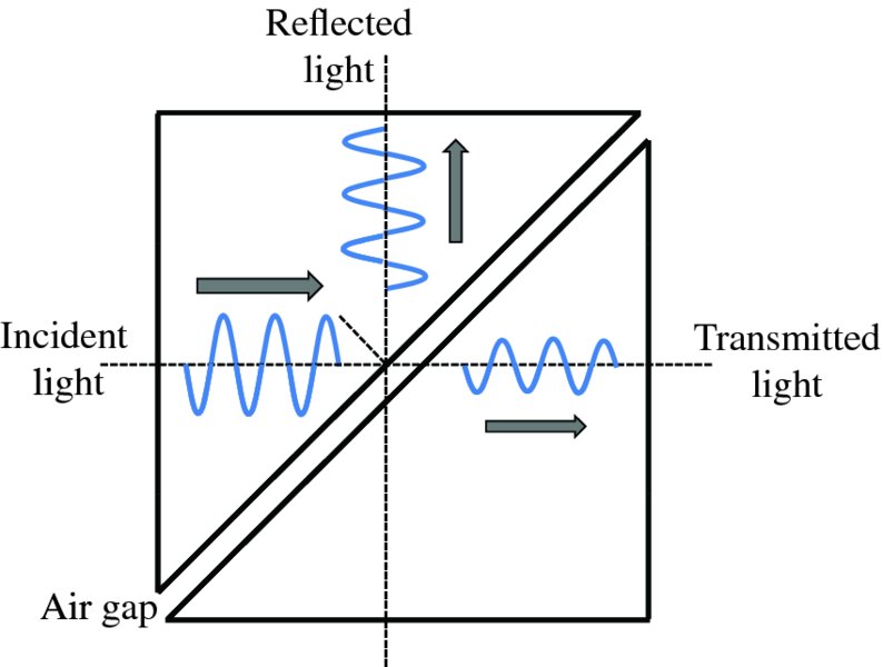
Figure 2.22 When light is incident upon the glass/air interface of a prism at an angle greater than the critical angle, it is totally internally reflected. However, because of its wave nature, the light can penetrate an air gap and pass into a second prism when the gap is of the order of the wavelength of the light. The critical angle for glass of refractive index 1.5 is 42°.
To determine the wave function in the three regions of the potential energy function shown in Figure 2.21, we proceed as before by solving Schrödinger's equation for each region and matching the wave function and their derivatives at x = 0 and x = L. This is fairly involved mathematically.3 What we find is that in the regions x < 0 and x > L, the wave functions exhibit an oscillatory behaviour (cf. Equation 2.33) while in the region 0 ⩽ x ⩽ L, the wave function has an exponential form (cf. Equation 2.42). The resulting wave functions are illustrated in Figure 2.21. The probability T that the particle tunnels through the barrier is proportional to the square of the ratio of the amplitudes of the wave functions to the left and to the right of the barrier. When the probability T is much smaller than 1, it is found that

where

There is a finite probability of the incident particle tunnelling through the barrier.
Moreover, the probability depends exponentially on the energy difference through the
term
 and on the barrier width L. This means that the probability is very sensitive to these parameters. Because of
the negative sign of the exponent, the probability decreases very rapidly with increasing energy difference (V0 − E) and increasing barrier width L.
and on the barrier width L. This means that the probability is very sensitive to these parameters. Because of
the negative sign of the exponent, the probability decreases very rapidly with increasing energy difference (V0 − E) and increasing barrier width L.
Barrier penetration is of great importance for nuclear fusion. A fusion reaction can occur when two nuclei tunnel through the barrier due to their mutual electrostatic repulsion and approach each other sufficiently closely that the attractive nuclear force causes them to fuse together.
2.3 Radioactivity and nuclear stability
Natural radioactivity was discovered before the existence of the nucleus had been established. In all, there are about 2500 known nuclides, but less than 10% of these are stable against radioactive decay; the majority are unstable and decay to other nuclides emitting particles and high-energy electromagnetic radiation. The essential idea is that an unstable nucleus will decay to a nucleus that is more stable, by which we mean more tightly bound. The timescales for radioactive decay range from a tiny fraction of a second to billions of years. Of the radioactive nuclides, over 60 can be found in nature and indeed we are surrounded by natural radioactivity. It comes from the rocks and soil that make up the planet, from the building materials of our homes and even from the food we eat. For example, potassium is present in many of our foods and the 40K isotope of potassium constitutes the major radioactive nuclide in our bodies. Some of the naturally occurring radioactive nuclides in nature, such as 238U, originated in the interior of stars and still exist because their half-lives are comparable to the age of the Earth (the age of the Earth is ∼5 × 10⁹ years, while 238U has a half-life of 4.5 × 10⁹ years). Others exist because long-lived nuclides like 238U decay in a chain of separate steps and produce a range of radioactive nuclides in the process. Although these product nuclides may have short half-lives, they are being continually created from the long-lived parent nuclide. Natural radioactivity also arises from radioactive isotopes that are produced by high-energy cosmic rays that rain down upon the Earth. For example, cosmic rays interact with molecules in the atmosphere to produce the 14C isotope of carbon, which is used in the technique of radiocarbon dating.
Radioactive nuclides are also produced artificially in particle accelerators and nuclear reactors. For example, radioactive nuclides for nuclear medicine are produced by bombarding stable nuclides with energetic particles in a cyclotron. In one application the radioactive isotope 131I is used to identify and treat cancerous nodules in the thyroid gland. A minute amount of 131I is injected into the patient. The speed with which the isotope is concentrated in the thyroid is a measure of how well the thyroid is working. Furthermore, employing sophisticated imaging techniques, the γ radiation from the decay of 131I can be used to obtain an image of the thyroid, which can show up abnormalities in, for example, thyroid size. If cancerous nodules are discovered, they can then be destroyed by a larger dose of 131I. The half-life of 131I is about 8 days, so that long-term effects of nuclear radiation are avoided. In the case of nuclear reactors, some of the radioactive nuclides they produce have half-lives of many thousands of years. These must be isolated from biological systems for periods of the order 105–106 years and one of the challenges of nuclear energy is to store these radioactive products securely over such long timescales.
2.3.1 Segré chart of the stable nuclides
We can organise nuclides on a so-called Segré chart, named after the nuclear physicist Emilio Segré. Each nuclide is indicated by a point on the chart where its neutron number N (vertical axis) is plotted against its proton number Z (horizontal axis). The Segré chart for the stable nuclides is shown in Figure 2.23. The points corresponding to the stable nuclides follow a curve called the line of stability and define a rather narrow region of stability. Also included in the figure is the straight line N = Z.
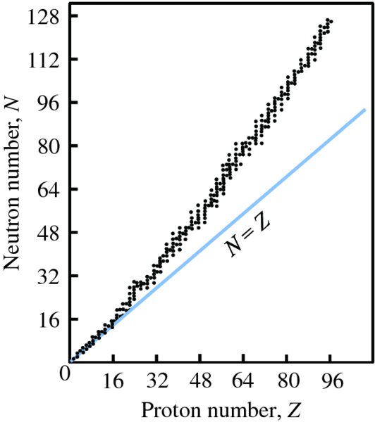
Figure 2.23 The Segré chart for the stable nuclides. Each nuclide is indicated by a data point, where its neutron number N is plotted versus its atomic number Z. Also shown is the straight line N = Z.
For Z less than about 16, we see that Z ≈ N. This is because, for light nuclei, the greatest stability is achieved when the number of neutrons and protons is approximately equal. For example, 4He, 12C and 16O all have the same number of neutrons and protons. For larger values of Z, N grows faster than Z and the ratio N/Z eventually reaches a value of about 1.6. This is because of the increasing influence of the electrostatic repulsion of the protons. We saw in Section 2.1.8 that nuclear binding energy is approximately proportional to A( = Z + N), while electrostatic repulsion energy is approximately proportional to Z 2, and of course a quadratic term increases faster than a linear term. The nuclear instability due to the electrostatic repulsion is minimised by having more neutrons than protons. The chart also reveals a tendency for stable nuclei to have even Z and even N. This tendency arises because two nucleons of the same species, either neutrons or protons, can couple together to form an especially strong bond. This makes a particularly large contribution to the nuclear binding energy, as we discussed in Section 2.1.8. 208Pb is the heaviest stable nuclide, although 209Bi has a half-life of 2 × 10¹⁹ years and can be considered to be stable for all practical purposes.
The Segré chart also reveals the various isotopes of the elements, which have the same Z but different values of N. The isotopes of a particular element have the same number of electrons and hence the same chemical properties. All these isotopes therefore fit into the same box in the periodic table of the elements. The nuclear properties of the isotopes of a given element are, however, generally quite different from one another.
In addition to the stable nuclides, there are the several thousand unstable nuclides. These have values of N and Z that lie outside the region of stability. They decay to stable nuclides, typically by α or β decay as described in Section 2.2.3.
2.3.2 Decay laws of radioactivity
Rutherford discovered that the number of radioactive nuclei in a sample decreases exponentially with time. This result is of practical importance. For example, we can use it to predict when a radioactive product from a nuclear reactor will have decayed sufficiently for it to be considered safe. The exponential time dependence is also of fundamental importance in that it indicates that radioactivity is a statistical process. We cannot predict how long a particular nucleus will survive before it decays. In a sample of uranium, for example, a particular nucleus may decay in the next second or it may not decay for a further billion years. On the other hand, we can say that about half the nuclei in the sample will decay within the half-life of the nuclide. For example, 2 mg of 238U contains approximately 5 × 10¹⁸ nuclei. Knowing its half-life, we can say that about 25 of these nuclei will decay each second. By analogy, when we toss a coin, we cannot predict whether the coin will turn up heads or tails. However, we can say that if we toss the coin 100 times, the number of heads will be close to 50.
The random nature of radioactivity was demonstrated by Rutherford and Geiger by observing the fluctuations of the number of α particles emitted by a particular source in a given time interval. For example, suppose we count the number of α particles that are emitted by a certain radioactive source in a fixed period of time, say 10 seconds, and we do this many times. We would find that the number of detected α particles would vary; sometimes it would be five counts say, sometimes four counts and sometimes seven counts, etc. The number would be random, although it would be within a limited range. The radioactive sample used by Rutherford and Geiger had a very long lifetime so that the nuclear activity could be assumed to be constant during the experiment. They plotted the number of times that n decays were recorded in the fixed period of time and they found that the distribution of n values was in agreement with the Poisson distribution for random events. The Poisson probability formula is
where P(n) is the probability for getting n counts in the counting period, m is the mean or average count rate and n! denotes the factorial function. (Happily, the mnemonic to remember the Poisson formula is the word ‘mnemonic’, i.e. m to the n times e to the minus m over n factorial.)
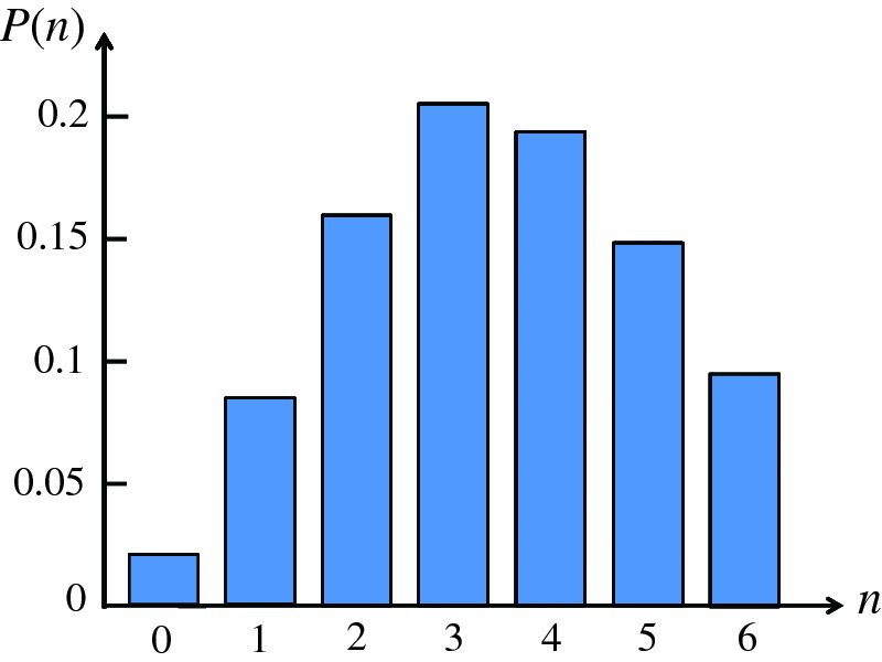
Figure 2.24 An example of a Poisson distribution where P(n) is the probability of n counts in a particular counting period. In this example the mean number of counts is 3.80.
Although we cannot say which particular nuclei in a sample will decay, we can say that if a sample contains N radioactive nuclei, then the rate ( = −dN/dt) at which nuclei will decay is proportional to N, as observed experimentally. The negative sign indicates the decrease in the number of radioactive nuclei. Hence we can write
where λ is called the decay constant. The left-hand side of this equation is the probability per unit time for the decay of a nucleus. That this probability is constant, regardless of the age of the nucleus, is the basic assumption of the statistical theory of radioactive decay. It readily follows that the probability that a given nucleus will decay in time dt is equal to λdt.
The observed, exponential decrease in the number of radioactive nuclei with time follows directly from the assumption of a constant probability per unit time λ for the decay of a nucleus. Thus, integrating Equation (2.51) from N = N0 at t = 0 to N at t = t, gives
The solution of this equation is
This is the familiar law of radioactive decay, and is the same for all forms of radioactive decay. Of course, the total number of nuclei in the sample does not change. The radioactive nuclei are simply converted into other, more stable nuclei. The half-life of a nuclide t1/2 is defined as the time it takes for half the nuclei to decay. Then,
giving
The number, N(t), of radioactive nuclei reduces by a factor of 2 for every half-life as illustrated by Figure 2.25, and after n half-lives the number remaining is (1/2)n N0.
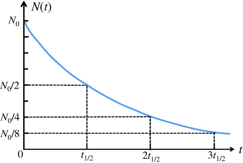
Figure 2.25 The exponential decay of the number N(t) of radioactive nuclei versus time t. N(t) reduces by a factor of 2 for every half-life t1/2.
Note that the number reduces by a factor of 2 every half-life, regardless of the instant of time we chose for t = 0. Clearly a nuclide will still be radioactive after one half-life, and indeed will remain so after several half-lives, although the decay rate will decrease.
In practice it is very difficult to measure the number of radioactive nuclei present
in a given sample. It is much easier to measure the number of radioactive decays per
unit time. This decay rate is called the activity
 and is simply the absolute value of dN/dt:
Hence, substituting for dN/dt from Equation (2.51):
giving
where
 is the initial activity at t = 0. We see that the activity also decays exponentially with time. When we plot the
natural logarithm of
is the initial activity at t = 0. We see that the activity also decays exponentially with time. When we plot the
natural logarithm of
 versus t, we obtain a straight line with a slope of − λ, as shown Figure 2.26. Hence, if we have experimental data for
 we can plot the data in this way to obtain the decay constant λ of the nuclide.
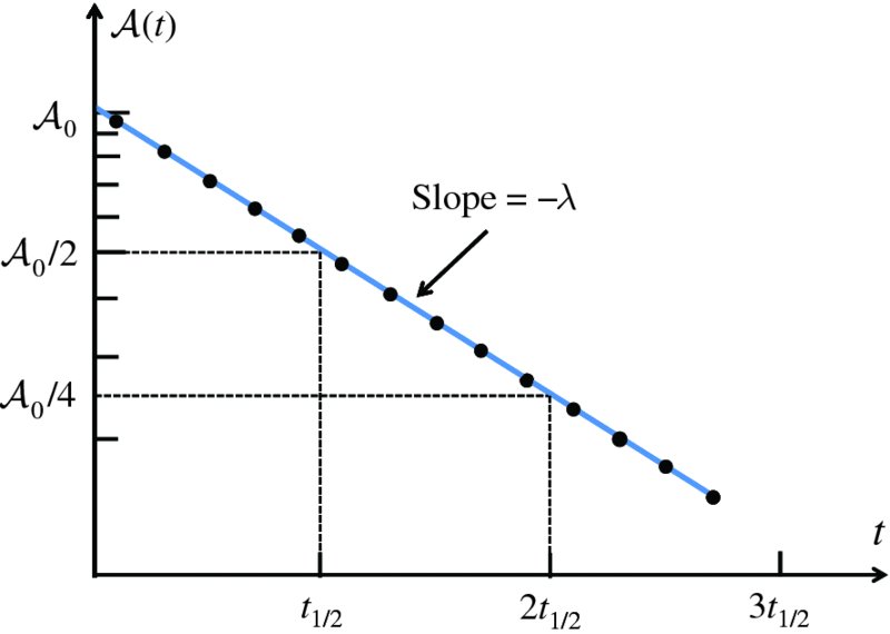
Figure 2.26 A semi-logarithmic plot of activity
 versus time t. The slope of the straight line is equal to −λ, where λ is the decay constant of the radioactive nuclide.
 reduces by a factor of 2 for every half-life t1/2.
The SI unit for activity is the becquerel (Bq), named after Antoine Henri Becquerel, where

However, a unit that is often used in practice is the curie (Ci), which is approximately the activity of 1 g of 226Ra. It is now defined as

The curie is a very large unit and laboratory sources are typically measured in millicuries
(mCi) or microcuries (μCi). Note that the activity
 of a source says nothing about the kind of particle or radiation emitted by the decaying
nucleus or the energy of the particles or radiation.
of a source says nothing about the kind of particle or radiation emitted by the decaying
nucleus or the energy of the particles or radiation.
Another useful parameter is the mean lifetime τ, which is defined as the average time that a nucleus is likely to survive before it decays. We can obtain the relationship between the mean lifetime and the decay constant λ as follows. The decay rate is equal to |dN/dt|. Hence, the number of nuclei that decay between t and t + dt is equal to
Figure 2.27 is a linear plot of
 versus t. The shaded area of the plot is
 and corresponds to the number of nuclei with lifetimes between t and t + dt. The sum of the lifetimes of these nuclei makes a contribution
 to the total sum of all lifetimes. Thus the total sum of the lifetimes of all the
nuclei is
to the total sum of all lifetimes. Thus the total sum of the lifetimes of all the
nuclei is
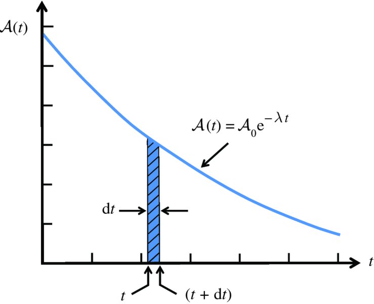
Figure 2.27 A linear plot of activity
 versus time t. The shaded area of width dt corresponds to the number of nuclei that have lifetimes between t and (t + dt).
Substituting for
 from Equation (2.57) and integrating the resultant integral, we obtain
As the total number of nuclei is N0, the mean lifetime τ is given by

We see that the mean lifetime τ is equal to the reciprocal of the decay constant λ. The mean lifetime is often simply called the lifetime of the nuclide. From Equations (2.55) and (2.61) we have

Decay chains
A common situation occurs for high mass number radioactive nuclides where the decay of a nucleus produces another radioactive nucleus. And indeed there may be a chain of radioactive decays, e.g. 238U → 234Th → 234U→ … → 206Pb. The original nucleus is called the parent nucleus and the succeeding generations are called its daughter, grand-daughter, etc. Suppose we have a parent A that decays to a radioactive daughter B that in turn decays to a stable grand-daughter C. At time t = 0, we have NA = N0, NB = NC = 0. We are interested in how NA and NB vary with time. We can say at once that the total number of nuclei will remain constant:

For nucleus A we have
with dNA = −λANAdt.
For nucleus B we have

This corresponds to the number of nuclei B produced in the decay of nucleus A minus the number decaying to nucleus C. This leads to the differential equation
Using the result
we obtain
We integrate this equation:
to give
Using the boundary condition, NB = 0 at t = 0 and simplifying we finally obtain an expression for the number of NB nuclei:
The quantity that is measured in practice is the activity
 , which is equal to λBNB:
The activity of the parent is
 . Hence, the ratio of activities is
If the parent is long-lived compared with the daughter, i.e. λA ≪ λB, the parent decays at an essentially constant rate, and
After a few mean lives τB of the shorter-lived daughter, the exponential term becomes negligible and the activity
of the daughter becomes equal to the activity of the parent:
 . This condition is called secular equilibrium.
This analysis can be readily extended to the case where there are many steps in the decay chain, where the daughter and succeeding generations have lifetimes that are short compared with the parent lifetime. It explains why radioactive nuclides with very short lifetimes are found in nature: the short-lifetime radioactive nuclei are in equilibrium in decay families with long lifetime parents.
2.3.3 α, β and γ decay
When an unstable nucleus decays to become a more stable nucleus, it may emit an α particle or a β particle. Furthermore, this may result in a daughter nucleus that is in an excited state, which then decays towards its ground state by emitting a γ-ray. Early on in the study of radioactivity it was discovered that α particles are bare helium nuclei, He++, that β particles are electrons (or positrons) and that γ-rays are highly energetic photons. Figure 2.28 illustrates the effect of a magnetic field on each of them, assuming they have equal energy. Being relatively light, negatively charged β particles suffer large deflections in the magnetic field. The much heavier and positively charged α particles are deflected by a much less amount and in the opposite direction. γ-rays are uncharged and are not deflected at all. These emissions that occur in radioactive decay are collectively called nuclear radiation.
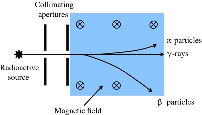
Figure 2.28 The behaviour of α particles, β− particles and γ-rays in a magnetic field, all having the same energy. The relatively light, negatively charged β− particles suffer large deflections in the magnetic field. The much heavier and positively charged α particles are deflected by a much smaller amount and in the opposite direction. The γ-rays are uncharged and are not deflected at all.
α, β and γ decay are the principal types of radioactive decay. However, it might be the case that a heavy radioactive nucleus decays to an unstable nucleus that has a large excess of neutrons and therefore lies very far from the region of nuclear stability. In that case, the unstable product nucleus will usually decay by emitting some of the excess neutrons. Importantly, the time that elapses before these neutrons are emitted may be relatively long, ∼ several seconds. We will see that these so-called delayed neutrons are crucial to the control of a nuclear fission reactor.
α decay
In α decay, a high-Z parent nucleus X decays to a daughter nucleus X' by emitting an α particle:
This lowers both the nuclear charge and the nuclear mass. It also liberates energy because the decay products are more tightly bound than the parent nucleus. And since the α particle has a relatively large binding energy, there is a correspondingly large energy release. This energy release, called the Q-value, is the energy equivalent of the mass defect of the reaction:

where, taking the mass of the electrons into account, MX, MX' and MHe are the atomic masses of the parent, the daughter and the helium atom. Clearly, it follows that α decay can only occur when the atomic mass of the parent is greater than the sum of the atomic masses of the daughter and of helium. The released energy is shared as kinetic energy between the daughter nucleus and the α particle and, as the α particle has the much smaller mass, it carries away most of the released energy.
A striking feature of α-particle decay is that the lifetimes of the nuclides that α decay vary enormously, while the kinetic energies of the emitted α particles lie within a rather narrow range; lifetimes vary from a tiny fraction of a second to ∼1010 years, while the kinetic energies lie between about 4 and 9 MeV. For example, 232Th has a half-life of 1.4 × 10¹⁰ years and emits an α particle with a kinetic energy of 4.08 MeV, while 218Th has a half-life of 1.0 × 10− 7 s and emits an α particle with a kinetic energy of 9.85 MeV. A factor of ∼2 in α-particle energy results in a factor of ∼1024 in half-life. These characteristics of α decay were explained by G. Gamow and independently by E. Condon and R Gurney in 1928 using quantum wave mechanics. They explained the paradox of α-particle emission in terms of barrier penetration, and in fact their successful application of quantum wave mechanics was one of its earliest and most convincing verifications.
Barrier penetration model of α decay
In the model of Gamow et al., it is assumed that the α particle, which as we have seen is a particularly tightly bound system, is pre-formed inside the parent nucleus. We then have the picture of the α particle moving in a spherical region that is determined by the daughter nucleus, which has a nuclear charge of (Z − 2). Figure 2.29 represents the potential energy function V(r) for the α particle as a function of its radial distance r from the centre of the daughter nucleus. Outside the nucleus, V(r) is the electrostatic potential:
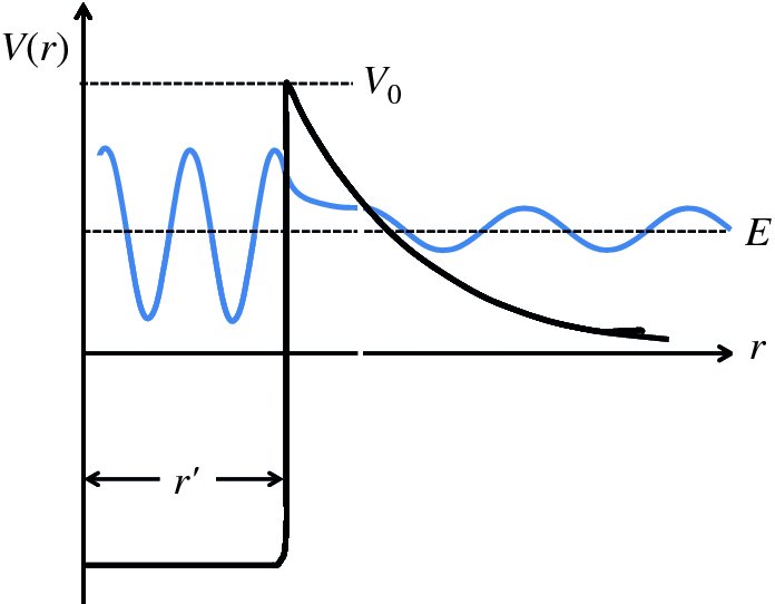
Figure 2.29 Potential energy function, V(r), for an α particle trapped inside a daughter nucleus, as a function of radial distance r. The radius r′ can be taken as the sum of the radius of the daughter nucleus and of the α particle. Outside the nucleus, V(r) is the potential due to the 1/r Coulomb repulsion between the α particle and the nucleus. Inside the nucleus, V(r) is represented by a square well, which reflects the potential energy due to the nuclear force. The horizontal line E represents the kinetic energy of the α particle at a large distance from the nucleus. The figure also shows schematically the wave function of the α particle. It is oscillatory inside the nucleus, decreases exponentially in amplitude within the barrier and becomes oscillatory again outside the nucleus. Quantum mechanically, the α particle has a finite probability of tunnelling through the Coulomb barrier.
where 2e is the charge on the α particle. Inside the nucleus V(r) is represented by a square well, which reflects the potential energy due to the nuclear force. This combination of electrostatic and nuclear potentials gives rise to a Coulomb barrier (see also Section 2.2.2). The horizontal line E represents the kinetic energy of the α particle at a large distance from the nucleus. If we assume that the daughter and α particle are uniformly charged spheres, we can estimate the electrostatic potential energy V0 when they are just touching, i.e. the height of the Coulomb barrier. This is given by

where r' is the sum of the radii of the daughter nucleus and the α particle. We can estimate
these radii using the relationship R = R0A1/3, with R0 = 1.2 × 10− 15 m. Taking the example of
 , we estimate r' to be

Taking this value for r′:
This value for the height of the Coulomb barrier is typical for nuclides that decay by α-particle emission. Clearly, it is much larger than the energies of emitted α particles, which are ∼5 MeV. Classically, therefore, α decay should not be possible. Quantum mechanically, however, there is a finite probability for the transmission of an incident particle through a potential barrier, as we saw in Section 2.2.3. For the case of a rectangular barrier, the probability T that the particle tunnels through the barrier is given by
where
although in the case of α decay, the exponential term dominates the behaviour of T so that it is sufficient to take

The Coulomb barrier, however, is not rectangular in shape, as can be seen in Figure 2.29. Gamow et al. therefore approximated the shape of the Coulomb barrier by a sequence of infinitesimally narrow rectangular barriers of height V(r) = 2(Z − 2)e2/4πϵ0r and width dr. This leads to the following expression for T:
which gives the probability that an α particle will tunnel through the Coulomb barrier when it is incident upon it. The energy E is the measured kinetic energy of the emitted particle because far from the nucleus its potential energy is zero. Figure 2.29 shows schematically the wave function of the α particle. It is oscillatory inside the nucleus, decreases exponentially in amplitude within the barrier and becomes oscillatory again outside the nucleus.
To determine the α decay rate, Gamow et al. assumed that the α particle bounces back and forth inside the daughter nucleus, hitting the barrier at the nuclear radius. Each time the α particle strikes the barrier there is a small probability, T, that it tunnels through the barrier and appears outside the nucleus. The number of times per second, N, that it strikes the barrier can be estimated from

where v is the velocity of the α particle and 2R the nuclear diameter. The value of v is assumed to be comparable to the velocity of the α particle after the emission. Then the decay rate of the nucleus will be ∼ N × T. For example, 238U decays to 234Th with the emission of an α particle of kinetic energy 4.20 MeV with a half-life of 1.42 × 10¹⁷ s. Taking the diameter of 234Th to be 2 × 2341/3 × 1.2 = 14.8 fm and the α particle to have a velocity in the nucleus of 1.42 × 10⁷ m/s, an α particle strikes the Coulomb barrier ≈ 1 × 10²¹ times/s. Hence it must make, on average, ∼1038 attempts before it finally escapes. So, although finite, the probability of tunnelling, T, is extremely small. Using their model, Gamow et al. obtained α-decay rates that were in good agreement with those measured experimentally.
The height, V0, of the Coulomb barrier and the nuclear radius, R, do not change significantly for nuclei in the limited range of the periodic table in which α-emitting nuclei are found. The enormous variation in α-decay rate from one nuclide to the next arises from the exponential dependence of the transmission probability T on [V(r) − E] and on L. As the energy E of the emitted α particle increases, the term [V(r) − E] decreases and the width of the barrier decreases as the α particle reaches higher up the barrier.
β decay
For a given value of mass number A there can be various possible combinations of atomic number Z and neutron number N. Some combinations result in more stable nuclides than others. Nuclides that have a combination of Z and N that is not the most stable may change these Z and N values, whilst retaining the same value of A by β decay. In a β-decay process, neutrons may be converted into protons or vice versa, bringing an unstable nucleus closer to the line of nuclear stability (see Figure 2.23). β decay can occur in three possible ways, each of which involves another charged particle to conserve electric charge:
The first process is known as β-minus decay, which involves the creation and emission of an electron and the conversion
of a neutron into a proton. The second process is called β-plus decay, which involves the creation and emission of a positron and the conversion of a proton into a neutron.
In the third process, a proton is again converted into a neutron but now an atomic electron from an inner-shell orbital is captured by the nucleus. In all three processes,
a further particle, called a neutrino
ν (or antineutrino
 ), is also emitted.
The force that governs β decay is the weak nuclear force. This is much weaker by a factor of ∼1012 than the nuclear force that binds nucleons together in a nucleus. It also has a much shorter range. Speaking in very general terms, we can say that if a force is weak, it takes a ‘long time’ to produce an effect. So the lifetimes for β decay tend to be long. For example, the half-life of 14C which β− decays is 5730 years.
β− decay
The simplest example of β− decay occurs for a free neutron:
The decay is energetically favourable because the mass of a proton is less than that of a neutron, by 0.001 388 4 u. Indeed, neutrons are unstable against β decay, with a half-life of 10.6 min. Free neutrons are produced in various nuclear reactions as we will see in Chapter 3. Such free neutrons are widely used to study materials, because the de Broglie wavelength of a thermal neutron, with a thermal energy kT of 1/40 eV, is about the same as the spacing of the atomic planes in a crystal. Usually, however, the neutron is bound in a nucleus and we have:
Note that the Z value increases by 1 and the N value reduces by 1 but the atomic number, A = Z + N, remains the same.
Electron emission can take place if the mass < ?TeX$AZm of the initial nucleus is greater than the mass
 of the final nucleus plus the rest mass me of the electron:

In terms of atomic masses AZM, and neglecting the binding energies of the atomic electrons

Hence, β− decay is allowed if

which reduces to the simple result:
β− decay can occur so long as the initial atomic mass is greater than the final atomic mass; the mass of the electron added to the atom is compensated by the mass of the electron emitted by the nucleus. The mass excess times c2 is the energy E made available in the decay:
An important example of β− decay is
which is used in radioactive carbon dating. As noted previously, the action of cosmic rays on atmospheric molecules produces 14C, and for every 1012 atoms of stable 12C there are about 1.5 atoms of 14C. Both of these isotopes are taken up in this proportion by living organisms such as plants and trees when they absorb carbon dioxide. When the organism dies, it stops taking in carbon. The 14C decays by β− emission to 14N with a half-life of 5730 years and hence the exponential decay of the 14C serves as a clock to measure the time from when the organism died. The technique of radioactive dating thus involves determining the relative amounts of the unstable 14C isotope and the stable 12C isotope in the remains of the organic matter. For example, if the number of 14C atoms was 1.5 per 1012 atoms of carbon at the moment an organism died, then that number would fall to 0.75 per 1012 atoms of 12C after 5730 years. This half-life of 14C is appropriate for measuring time intervals in the range of historical interest. The dating the Dead Sea scrolls is just one of many examples of the use of radioactive carbon dating. For much longer timescales, such as the age of rocks and that of planet Earth, radioactive nuclides with much longer half-lives are used. For example, the radioactive isotope 40K decays to 40Ar by electron capture with a half-life of 1.2 × 10⁹ years, and the age of a rock, for example, can be determined by measuring the ratio of 40K to 40Ar in the rock.
In the first experimental investigations of β− decay, the investigators were not aware of the emitted antineutrino and this led
to some puzzling observations. The electrons were found to have a continuous distribution of energy, as illustrated in Figure 2.30. This would not be possible if β−decay were a two-body process, as this would require the ejected electron to have
a definite energy, which was not observed. Furthermore, angular momentum could not
be conserved if the neutron and the proton were the only reaction products, as the
neutron, proton and electron are all spin-1/2 fermions. Since the neutron spin is 1/2, the resulting total proton-electron spin can only be either 0 or 1. The answer to
these puzzling results came in 1931 when Wolfgang Pauli postulated the existence of
a third body to take away the excess energy and conserve linear and angular momentum.
For conservation of charge, this body must be electrically neutral, and from conservation of angular momentum, it must be a spin-1/2 particle. Moreover, the maximum energy of the ejected electron in the β− decay was found to be equal to the decay energy E within the experimental uncertainty. This implied that the mass of the third particle
must be zero or nearly zero. The third particle that Pauli postulated is the antineutrino
 . Now it is believed that the neutrino has a finite but exceedingly small mass. The
fact that the antineutrino was not observed in the experiments implies, correctly,
that it is not affected by nuclear or electrostatic forces. Indeed, antineutrinos
(and neutrinos) hardly interact with matter at all. Many millions of neutrinos pass
straight through our bodies every second, while a neutrino can readily pass through
the universe without interacting. It is not surprising therefore that antineutrinos
are very hard to detect, and indeed it was nearly 30 years after Pauli's postulation
of their existence that they were detected experimentally.
. Now it is believed that the neutrino has a finite but exceedingly small mass. The
fact that the antineutrino was not observed in the experiments implies, correctly,
that it is not affected by nuclear or electrostatic forces. Indeed, antineutrinos
(and neutrinos) hardly interact with matter at all. Many millions of neutrinos pass
straight through our bodies every second, while a neutrino can readily pass through
the universe without interacting. It is not surprising therefore that antineutrinos
are very hard to detect, and indeed it was nearly 30 years after Pauli's postulation
of their existence that they were detected experimentally.
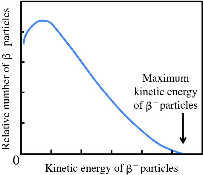
Figure 2.30 The continuous distribution of kinetic energy for β− particles emitted in the β− decay of a radioactive nuclide. The vertical arrow indicates the maximum kinetic energy that a β− particle can have.
β+ decay
We represent a β+ decay process as

The number of protons Z reduces by 1 and the number of neutrons N increases by 1, but the atomic number A remains the same. For β+ decay to occur, the proton must be bound in a nucleus, as the decay of a free proton
is energetically forbidden. In a similar way to the above, it can be readily shown
that for β+ decay to occur, the original atomic mass must be greater than the final atomic mass
by at least two electron masses:
 .
.
An important aspect of β+ decay is that it provides a source of positrons, which are required in a range of applications. For example they are used in positron emission tomography (PET), which is an imaging technique that produces a three-dimensional image or picture of functional processes in the body. The positrons collide with electrons in the body, producing annihilation radiation that is detected by a camera.
Electron capture
An alternative to β+ decay is electron capture where a nucleus captures one of its atomic electrons, with the result that a proton in the nucleus is transformed into a neutron and a neutrino is emitted:

The captured electron usually comes from the innermost (n = 1) orbit of the atom as this orbit is closest to the nucleus and the overlap of the electronic wave function with the volume of the nucleus is greatest. The vacancy
is soon filled by an electron from a higher lying orbit, which results in the emission
of an X-ray. The wavelength of the X-ray is characteristic of the daughter nucleus. As the electron is provided by the atom, electron capture can occur if the
original atomic mass is greater than the final atomic mass:
 . Hence, there is a range of unstable nuclides where the difference in atomic masses
is such that electron capture is allowed but β+
decay is energetically forbidden.
. Hence, there is a range of unstable nuclides where the difference in atomic masses
is such that electron capture is allowed but β+
decay is energetically forbidden.
γ decay
Most α and β decays, and also most nuclear reactions, leave the final nucleus in an excited state. These excited states decay rapidly towards the ground state via the emission of one or more γ-rays, typically within a timescale of <10− 9 s. The process is analogous to the way atoms in excited states decay back to their ground state, but the energies and wavelengths involved are very different. Since energy spacings in nuclei are ∼MeV, γ-rays have wavelengths of ∼10− 12 m, about 106 times shorter than visible light. Unlike α or β decay, neither the mass number A nor the atomic number Z changes during γ decay.
An important example of γ decay occurs in the decay of the radioactive isotope of caesium, 137Cs, which is a fission product in the radioactive decay of 235U. The 137Cs isotope β decays to 137Ba and leaves the 137Ba nucleus in an excited state, denoted as 137Ba*:

as illustrated in Figure 2.31. This excited state lies 0.66 MeV above the ground state of 137Ba and decays to it with the emission of a γ-ray of this energy:
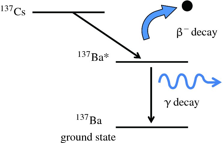
Figure 2.31 A 137Cs nucleus may decay to a 137Ba nucleus with the emission of a β− particle, leaving the 137Ba nucleus in an excited state, labelled 137Ba*. The excited 137Ba nucleus then decays to its ground state with the emission of a γ-ray. The energy of the γ-ray is equal to the energy difference (0.66 MeV) between the excited and ground states of the 137Ba nucleus.
Through these reactions, the 137Cs isotope provides an important laboratory source of γ-rays and finds application, for example, in radiation therapy in medicine. But note that the γ-rays are emitted by the 137Ba nucleus and not by the 137Cs nucleus.
Problems 2
-
When an excited state of the 137Ba nucleus decays to the ground state of 137Ba, it emits a γ-ray of energy 0.66 MeV. Calculate the wavelength and frequency of the γ-ray.
-
(a) Determine the nuclear radius and estimate the nuclear density of the following nuclides:
 , 5626Fe and
 . Compare these densities with the typical density of a neutron star. (b) Show that
the density of nuclear matter is roughly constant and independent of mass number A. (c) Estimate the charge density for the above nuclides. Comment on your results.
. Compare these densities with the typical density of a neutron star. (b) Show that
the density of nuclear matter is roughly constant and independent of mass number A. (c) Estimate the charge density for the above nuclides. Comment on your results.
-
Calculate the total binding energy of the
 nuclide. Compare its mass defect with the total mass of the atom, which is 119.902
197 u. What is the binding energy per nucleon?
nuclide. Compare its mass defect with the total mass of the atom, which is 119.902
197 u. What is the binding energy per nucleon?
-
(a) An α particle is taken apart in the following steps: (1) a proton is first removed; (2) then a neutron is removed; and (3) the remaining proton and neutron are separated. Determine the energy required for each step. Compare your results with the total binding energy of an α particle. (b) Determine the amount of energy it takes to remove a neutron from an α particle. Comment on your result with respect to step (1) in part (a). The atomic and neutron masses are:
-
The following table gives the binding energy per nucleon B/A for a range of nuclides. Plot the values of B/A versus A for these nuclides and on this plot make a sketch of the binding energy curve. Use your curve to estimate the value of B/A for 119Pd. Suppose that a nucleus of 238U were to fission into two 119Pd nuclei. Estimate the energy that would be released in this process.
Nucleus 2D 4He 7Li 9Be 12C 16O 40Ar 56Fe 98Mo 127I 181Ta 238U B/A(MeV) 1.11 7.07 5.61 6.46 7.68 7.98 8.60 8.79 8.64 8.45 8.02 7.57 -
For a given value of mass number A there may be various values of atomic number Z. Use the semi-empirical mass formula to show that the value of Z that gives the most tightly bound nucleus, i.e. the one with the smallest mass, is given by
What is the most stable nuclide with A = 121?
-
(a) Determine the Coulomb force (in N) between the two protons in an α particle assuming they are a distance 2 fm apart. (b) By what factor is the Coulomb force greater than the gravitational force between the two protons? (c) The energy required to separate all four nucleons in an α particle is about 28 MeV. Show that the nuclear force between two nucleons is ∼520 N by considering the range of the nuclear force.
-
Given that 1.0 g of 226Ra has a nominal activity of 1 Ci, find the half-life of 226Ra. Marie and Pierre Curie are said to have amassed 200g of 226Ra by 1900. How much of that 226Ra remained in 2000?
-
The table below shows measurements of the activity
 of a sample of
128I. Plot the data as a semi-log graph of
of a sample of
128I. Plot the data as a semi-log graph of
 versus time t and deduce the decay constant λ and the half-life
t1/2 of
128I.
versus time t and deduce the decay constant λ and the half-life
t1/2 of
128I.
Time, t (min) 0 25 50 75 100 125 150 175 200  (counts/s)
950 475 238 119 59 30 15 7.4 4.0 -
The total number of detected α particles from a sample of 238U is found to be 25 056 in a counting period of exactly 24 hours. Suppose that we do an experiment where we measure the number n of α particles that are counted in a period of 10 s and we do this a large number of times. Construct the Poisson distribution to which you could compare the experimental data. Take values of n from 0 to 4. What is the probability that more than four counts are recorded in a period of 10 s? What is the probability that at least one count is recorded in a period of 10 s? What does the fact that the detected counts follow a Poisson distribution tell us about the nature of radioactive decay?
-
A radioactive nuclide A decays to a daughter nuclide B that in turn decays to a stable nuclide C. Suppose that, initially, the number of A nuclei is 1000, the half-life of nuclide A is 10 min and the half-life of nuclide B is 1 min. Write a spreadsheet program to plot the populations NA, NB and NC against time t, on the same graph. On another graph, plot the activities
 of nuclides A and B against t. Investigate other combinations of half-lives.
-
(a) Show that carbon in the atmosphere has an activity of 15.6 decays/min/g. The relative abundances of stable 12C and radioactive 14C in the atmosphere are in the ratio 1:1.35 × 10⁻¹² and the half-life of 14C is 5730 years. (b) A 250 g sample of charcoal from an ancient fire is found to produce a β− decay rate of 500 decays/min. How old is the charcoal?
-
(a) What nuclide is produced in the following radioactive decays? (i) α decay of
 , (ii)
β− decay of
2411Na13, and (iii)
β+ decay of
, (ii)
β− decay of
2411Na13, and (iii)
β+ decay of
 . (b) What particle (alpha, electron or positron) is emitted in the following radioactive
decays: (i)
2714Si → 1327Al (ii)
. (b) What particle (alpha, electron or positron) is emitted in the following radioactive
decays: (i)
2714Si → 1327Al (ii)
 ; and (iii)
7433As → 3474Se?
; and (iii)
7433As → 3474Se?
-
(a) A stationary nucleus decays by α particle emission. Show that the kinetic energy of the recoiling daughter nucleus is equal to 4Q/A to a good approximation, where Q is the energy release and A is the mass number of the daughter. Obtain the corresponding expression for the kinetic energy of the α particle. (b) A potential hazard in homes in some geographical areas is the radioactive gas radon-222, which is produced by the α decay of radium-226. Determine the velocities of the emitted α particle and the recoiling daughter nucleus for this decay. The atomic masses of 226Ra, 224Rn and 4He are 226.025 406, 222.017 571 and 4.002 603 u, respectively.
-
 may α decay to
 or there is a very small probability that it may decay to
 by emitting a
 nucleus. Show that both processes are energetically possible and compare the Coulomb
barriers for the two processes. Comment on your results. The atomic masses of
nucleus. Show that both processes are energetically possible and compare the Coulomb
barriers for the two processes. Comment on your results. The atomic masses of
 ,
,
 ,
42He and
,
42He and
 are
223.018 501,
219.009 485,
4 002 603 and
14.003 242 u, respectively.
are
223.018 501,
219.009 485,
4 002 603 and
14.003 242 u, respectively.
-
(a) Show that β− decay of 6027Co to 6028Ni is energetically possible and find the maximum energy in MeV of the neutrino produced in the decay. The atomic masses of 6027Co and 6028Ni are 59.933 820 and 59.930 788 u, respectively. (b) Is it allowed energetically for a free proton to decay to a free neutron?
-
Show that 5727Co cannot β+ decay, but can decay by electron capture. The atomic masses of 5727Co and 5726Fe are 56.936 294 and 56.935 396 u, respectively. The mass of an electron is 5.4858 × 10− 4 u.
-
Plutonium-238 is an emitter of α particles of energy 5.59 MeV. This isotope has been used as a power source in spacecraft, where the energy of the emitted α particles is absorbed in a container surrounding the plutonium. Assuming that 10% of this emitted energy can be converted into electrical energy, what mass of plutonium is required to generate an electrical power of 1.5 W? The half-life of plutonium-238 is 87.7 years.