6
Wind power

We have already seen that the Sun delivers a huge amount of energy to the Earth's surface. Approximately 2% of this is converted into wind energy. This is a small fraction but still amounts to a global wind power of ∼2 × 10¹² kW. The purpose of wind turbines is to harvest some of this power. A wind turbine as described in this chapter is a machine that converts wind power into electricity, usually to supply electricity to a national grid. This is in contrast to a windmill, which converts wind power into mechanical power. Wind power has important advantages. It is a renewable energy source and it is also a clean source; it does not release harmful gases into the environment. Moreover, wind turbines can deliver power to remote areas that are not connected to a national grid. The main disadvantage is, of course, that the wind is variable and so is an intermittent source of energy. This means that wind turbines must be used in conjunction with other energy sources and/or energy storage systems. Nevertheless, because of its advantages, it is anticipated that wind power will in the future contribute at least 20% of global energy requirements.

In this chapter we describe the origin and directions of the wind and how a wind turbine works. As we are dealing with the flow of air, a fluid, through the blades of the turbine, it is also appropriate to introduce the physics of fluid flow. However, we first give a brief history of wind power.

6.1 A brief history of wind power

The use of wind power has a long history that goes back thousands of years. The first known historical reference is from the Greek mathematician and engineer Hero of Alexandria (c. 10–70 AD). He described a windmill that provided air to drive a musical organ. (Hero of Alexandria is also credited with the invention of the first steam engine.) In the following centuries the main use of wind power was to perform mechanical work. Holland, a flat and windy country, is famous for its use of windmills. They were used to pump water out of low lands and back into rivers beyond dikes so that the land could be farmed. The windmills were also used for many other purposes, including grinding grain for food and sawing logs. Similarly, the plains of America were made fertile by the use of windmills, which were used to pump underground water from beneath the plains to irrigate the fields. Wind continued to be a major source of energy up until the Industrial Revolution, but then began to recede in importance. Coal-driven steam engines had important advantages that the wind did not posses, such as portability and reliability of fuel supply.

Then, in 1831, the British scientist Michael Faraday succeeded in producing a current by moving a wire in a magnetic field. Faraday's law states that the induced electromotive force (emf), ϵ, in a closed circuit is equal to minus the rate of change of the magnetic flux ϕ through the circuit:

(6.1)

This discovery of electromagnetic induction was the beginning of electrical engineering. It led to the development of electrical generators that used electromagnetic induction to produce both DC and AC electrical power. These generators enabled the rotating mechanical motion of a wind turbine to be turned into electrical energy. In 1888, the American inventor Charles Brush built the first automatically operated turbine for the production of electricity. Bush's turbine had a rotor consisting of 144 blades of cedar wood with a diameter of 17 m. The turbine produced 12 kW of electrical power and Bush used the electricity to charge batteries that, in turn, powered the lights in his house. So he also took into account the fact that wind turbines, which depend on the availability of wind, require the storage of part of the energy produced. Bush's wind turbine system embodied many of the features of the future generations of wind turbines.

The latter part of the 19th century and the first half of the 20th century saw the construction of a number of larger wind turbines, which greatly influenced the development of today's technology. Probably the most important developments occurred in Denmark. In particular, Poul la Cour (1846–1908) was a Danish scientist and pioneer of wind power. He built the first wind tunnels for the purpose of aerodynamic tests to identify the best shape for turbines blades and he also investigated ways in which the energy from wind turbines could be stored. By the late 1960s people were becoming more aware of the environmental consequences of industrial development and this was followed by the mid-1970s’ oil crisis. This gave a new impetus to the development of wind power so that, by the end of 2015, the total installed capacity of wind power in the world was greater than 400 GW. Commercial wind turbines now have output powers in the range 1.5–8 MW.

6.2 Origin and directions of the wind

Wind is the movement of air from a region of high pressure to a region of low pressure; the larger the difference between the high and low pressures, the greater the wind speed. Pressure differences arise due to the rising and sinking of air in the atmosphere. Where air is rising, we get lower pressure at the Earth's surface, and where it is sinking we get higher pressure. The regions around the equator are heated by the Sun more than those regions around the poles for the geometric reasons we described in Section 4.3.2. Hot air is lighter than cold air and at the equator the air rises high into the atmosphere, producing a region of low pressure. This process pushes the air at the top of the atmosphere towards the north and south poles. As this air reaches colder regions, it starts to sink back to Earth where the pressure increases. If the Earth did not rotate, we would expect that the air would simply arrive at the north and the south poles, sink down and return to the equator, which is at a lower pressure, as illustrated in Figure 6.1. This would generate winds near the Earth's surface that travel from the poles back to the equator. In practice, however, this does not happen. This is because the direction of the wind is strongly influenced by the Earth's rotational motion. This rotational motion causes winds in the northern hemisphere to be deflected towards the right of their direction of travel, while winds in the southern hemisphere are deflected towards their left. This effect is described in terms of the so-called Coriolis force.

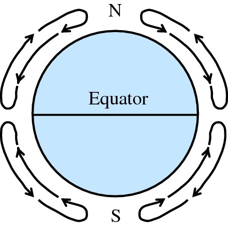
Figure 6.1 Circulation of the Earth's atmosphere in the absence of the Coriolis force. The air rises at the equator, producing low pressure there, and sinks at the colder poles, giving high pressure there.

6.2.1 The Coriolis force

Imagine that we launch a rocket from the north pole towards the equator and view its trajectory from outer space. Imagine also for a moment that planet Earth does not rotate about its axis. The rocket's trajectory that we would see is shown in Figure 6.2(a) and the rocket would land at point A on the equator. But Earth does rotate. So while the rocket is flying through the air, the point A on Earth is also moving; in an easterly direction at 465 m/s. Thus when the rocket lands, it does so at a point that is to the west of point A, as shown in Figure 6.2(b). For an observer located close to A, the rocket has apparently been deflected towards the west, i.e. towards the right with respect to its direction of travel. The apparent bending force is called the Coriolis force. The Coriolis force is not a true force like the force of gravity. It simply arises when an object moves in a rotating frame of reference, and is sometimes described as a pseudo force. It is named after the French scientist, Gaspard-Gustave Coriolis, who studied the transfer of energy in rotating systems.

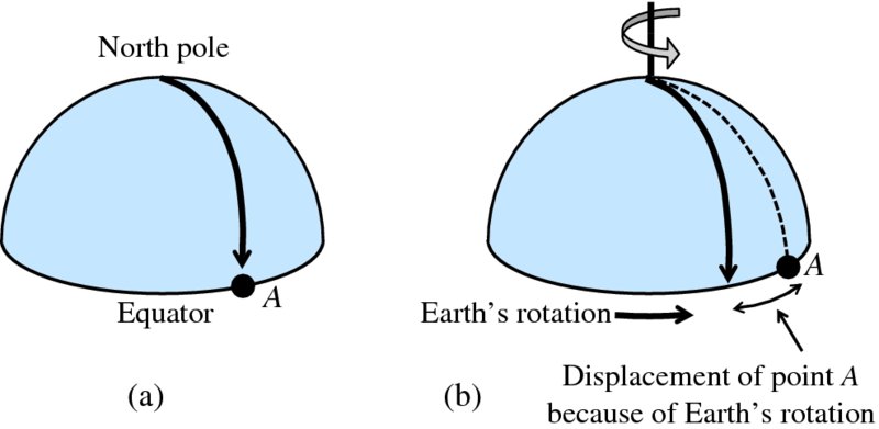
Figure 6.2 (a) The trajectory of a rocket in the northern hemisphere if the Earth did not rotate. (b) The trajectory of the rocket as the Earth does rotate. For an observer at point A, the rocket is deflected to the right of its direction of travel because of Earth's rotation.

An object moving in a northerly direction in the northern hemisphere is also deflected towards the right because of the Earth's rotation. We can see this as follows. Suppose that we now launch a rocket from the equator towards the north pole, as illustrated by Figure 6.3(a). While it is on the ground, the rocket is moving along with the Earth in an easterly direction at a speed u_east of 465 m/s. At its launch, the rocket is given a component of velocity u_north in the northerly direction, but it maintains its velocity component u_east in the easterly direction. The angular velocity, Ω, of the Earth about its axis is the same for all latitudes, of course. However, the linear velocity (r × Ω) of a given point on the surface of the Earth reduces as latitude increases, r being the perpendicular distance to the axis of rotation. The linear velocity is largest at the equator. So as the rocket travels to higher latitude, its component of velocity u_east parallel to the equator becomes greater than the speed of the ground beneath it. Hence, looking at Figure 6.3(b), we see that while point A, at a particular latitude, has moved a certain distance east since the rocket launch, the rocket has moved a greater distance to the east, given by point B. Again, to an observer close to point A it would appear that the rocket is deflected to the right. Similar considerations show that an object travelling in the southern hemisphere is deflected towards the left of its direction of travel.

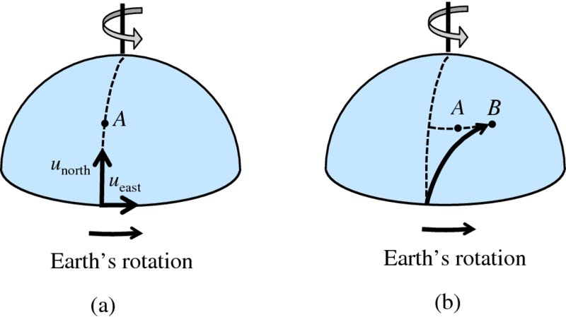
Figure 6.3 (a) The velocity components of a rocket that is fired in a northerly direction. (b) The rocket is deflected to right of its direction of travel according to an observer at point A because of the Earth's rotation.

The Coriolis force similarly affects the apparent direction of the wind. In the northern hemisphere, winds are deflected towards the right and in the southern hemisphere they are directed towards the left. This has profound consequences. The air flow that starts above the equator and travels at high altitude towards the north pole is deflected to the right by the Coriolis force. By the latitude of approximately 30°, the Coriolis force prevents the air from moving much further north and the air sinks to the Earth's surface. This leads to high pressure at that latitude; higher than the pressure at the equator. This sets up a cell of circulating air called the Hadley cell, as shown in Figure 6.4, where the arrows indicate the directions of the circulating air. This cell is named after George Hadley, an English lawyer and amateur meteorologist who proposed the mechanism by which winds are sustained. There are also two other such cells, called the Ferrel and the polar cell, as shown in Figure 6.4. These circulating currents of air produce the winds in the lower atmosphere. These winds are also affected by the Coriolis force; winds moving a northerly direction are deflected to the right and those moving a southerly direction are deflected to the left. This gives rise to the global wind pattern illustrated in Figure 6.4, which shows the well-know trade winds and westerlies. This pattern explains why, for example, the prevailing winds across the UK are west to southwesterly. At the junction of two cells, the horizontal wind speed is relatively small; most of the movement of the air is in the vertical direction. Thus, for example, in the region around the equator where the two Hadley cells meet, there is a region called the doldrums. This region was infamous among 18th-century sailors because of its calm wind conditions. The heights of the atmosphere in Figures 6.1 and 6.4 are greatly exaggerated. We saw in Section 5.3.3 that the height of Earth's atmosphere is ∼10 km. If we were to imagine Earth to be the size of an orange, the extent of the atmosphere would be less than 0.1 mm.

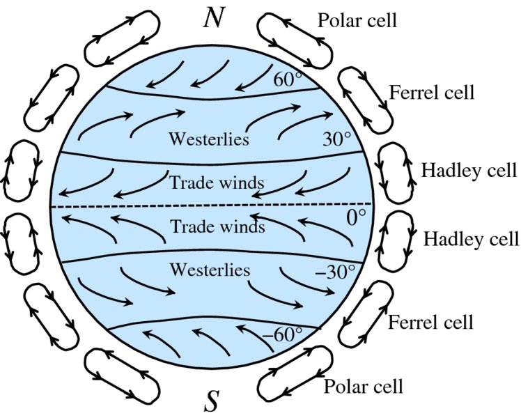
Figure 6.4 The cells of circulation in the atmosphere caused by the Earth's rotation, and the directions of the resulting global winds.

Although these global winds are of much importance in determining the prevailing winds at a particular location, local climatic conditions and landscape also influence wind direction. Again this involves the rising and sinking of air in the atmosphere. One of the simplest examples of a local wind is a sea breeze, which occurs where the land meets the sea. On sunny days, solar radiation heats the land quite quickly. By contrast, the sea is slower to warm up because it has a higher heat capacity. This leads to a temperature difference between the warm land and the cooler sea. As the land heats up, it warms the air above it, leading to lower pressure over the land. The air over the sea remains cooler and denser and so the pressure is higher than inland. This pressure difference produces a sea breeze blowing from the sea to the land. Clearly, the directions of the prevailing wind and local winds form a major consideration in the siting of wind turbines.

6.3 The flow of ideal fluids

The flow of a fluid can be extremely complex, as is evident in the rapids of a fast-flowing river. However, some systems of fluid flow can be represented by a relatively simple, idealised model. Moreover, in many situations we can often treat the fluid as an ideal fluid. This is a fluid that is (i) incompressible and (ii) has no viscosity, which means no internal friction. Liquids are essentially incompressible, but we can also treat gases as incompressible if the pressure difference from one region to another is not too great. And in many cases the frictional forces in the fluid can be neglected compared with forces arising from pressure differences or gravity.

A practical way to visualise the flow of a fluid is to inject dye into the fluid through a series of narrow, equally spaced channels so that the dye enters parallel to the direction of flow; if the fluid is air, smoke can be used instead. Figure 6.5 illustrates schematically what would be observed for the flow of a fluid past a cylinder. If the overall pattern of lines does not change with time, as in Figure 6.5(a), the die traces out a set of smooth and continuous lines. This is called steady flow and the lines are called streamlines. A streamline can be thought of as the path that a particle would take if placed in a flowing fluid. Thus a streamline is a curve whose tangent at any point is in the direction of the fluid velocity at that point. Note that all particles that pass through the same point follow the same path, i.e. the same streamline. Streamlines never intersect; no fluid particle can move across from one streamline to another. At the far left of Figure 6.5(a) the streamlines are parallel and horizontal. As they approach the cylinder the streamlines curve around the cylinder, getting closer together at the top and bottom of the cylinder. Then they spread out again before becoming parallel again at the far right. The flow pattern shown in Figure 6.5(a) is typical of laminar flow, where adjacent layers of fluid slide smoothly past each other. At sufficiently high flow rates or when obstacles cause abrupt changes in fluid velocity, the flow can become irregular and chaotic. This is called turbulent flow and the flow pattern changes continuously, as illustrated by Figure 6.5(b). In turbulent flow, the kinetic energy of the fluid is dissipated as thermal energy. Clearly turbulent flow has to be minimized as far as possible in the harvesting of energy from the wind.

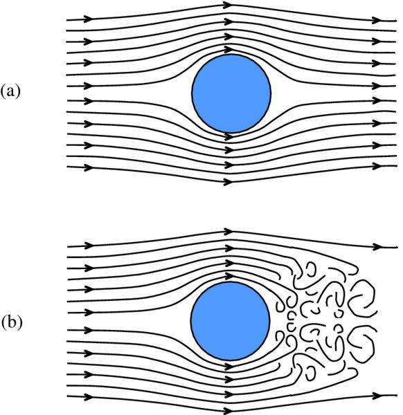
Figure 6.5 Schematic for the flow of a fluid past a cylinder. (a) Steady or laminar flow, where the overall pattern of streamlines does not change with time; the streamlines curve around the cylinder becoming closer together at the top and bottom of the cylinder. (b) Turbulent flow where the flow pattern changes continuously, making it irregular and chaotic.

6.3.1 The continuity equation

Imagine now that a fluid travels down a pipe of decreasing cross section as shown in Figure 6.6, where the fluid flows from left to right. The shaded volume on the left depicts the volume ΔVof fluid that flows through area A₁ in time Δt. If the speed of the fluid is u₁, the volume, ΔV, is given by:

(6.2)

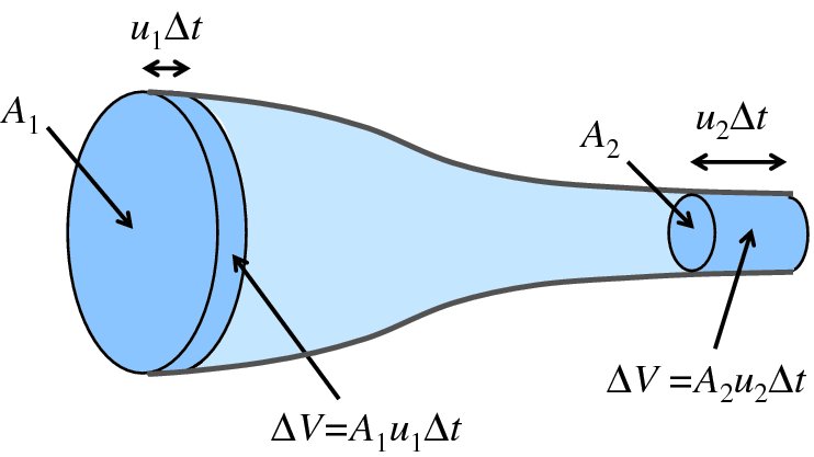
Figure 6.6 The figure shows a fluid that flows from left to right down a pipe of decreasing cross-section. The shaded volume on the left depicts the volume of fluid that flows through area A₁ in time Δt. The volume that flows through area A₂ in time Δt is depicted by the shaded area on the right. These volumes must be equal according to the continuity equation.

We assume that the fluid is incompressible so that an equal volume of fluid must flow past any point along the pipe during the same time, Δt. The volume that flows through area A₂ is depicted by the shaded area on the right of Figure 6.6. If the speed of the fluid is u₂ at A₂ this volume of fluid is equal to A₂u₂Δt. As these volumes must be equal we have

(6.3)

so that

(6.4)

This is a continuity equation, where the quantity (Au) is called the volume flow rate. We see that Au is a conserved quantity. We also have Δm = ρΔV, where ρ is the density of the fluid and Δm is the mass of fluid in volume ΔV. Hence we can write

(6.5)

giving

(6.6)

where we denote dm/dt as . As Au is a conserved quantity, is also a conserved quantity for constant density ρ; the mass flow is the same across any cross-sectional area of the pipe.

6.3.2 Bernoulli's equation

A fluid will flow between two different regions if there is a pressure difference between them. The resulting force on the fluid due to this pressure difference causes the fluid velocity to increase. It is Bernoulli's equation that relates the pressure and velocity of a fluid at a particular point.

Imagine a particular streamline in a steady flow situation as shown in Figure 6.7. And imagine a very small cube of fluid moving along this streamline with velocity u = ds/dt, where distance s is measured along the streamline. The inset on the figure shows an enlarged view of the front face of this cube, which has length l. The pressure p will, in general, vary along the streamline, as also will the velocity u of the cube. If p is the pressure at the centre of the cube, the pressure acting on the left face of the cube can be expanded as [p − (dp/ds)l/2] when l is small. Similarly, the pressure acting on the right face of the cube can be expanded as [p + (dp/ds)l/2].

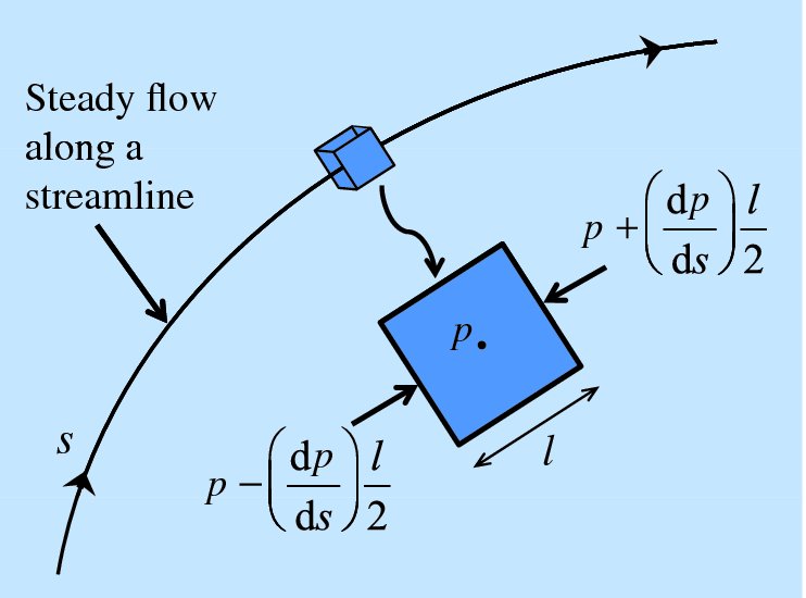
Figure 6.7 A very small cube of fluid moving along a particular streamline with velocity u = ds/dt. The inset shows an enlarged view of the front face of this cube, which has length l. The pressure p will, in general, vary along the streamline, as also will the velocity of the cube.

Hence, the net force acting on the cube of fluid along the s-direction is

Then, applying Newton's second law, we obtain

(6.7)

where ρ is the fluid density. Simplifying this equation gives

(6.8)

As velocity u is a function of s, we have

This gives

where we have used d(u²) = 2udu. Then, integrating along the streamline from pressure p₁ to p₂, we have

Hence,

(6.9)

which we can also write as

(6.10)

Equations (6.9), and (6.10) are expressions of Bernoulli's equation. Notice, in particular, that Bernoulli's equation says that as the pressure p reduces, the velocity u must increase. This result was first expressed in words by the Swiss mathematician Daniel Bernoulli in 1738 and was later derived in equation form by his associate Leonard Euler in 1755. Bernoulli's equation is much used in situations of fluid flow where compressibility and viscosity can be ignored.

Pressure can be thought of as potential energy per unit volume, as we will see further in Section 8.2.2. This is evident from the dimensions of both these quantities: [ML^-1T^{− 2}]. Hence the quantity p/ρ is potential energy per unit mass. And we can recognise the quantity u²/2 as kinetic energy per unit mass. Hence, Bernoulli's equation is simply a statement of the conservation of energy.

---

Worked example

Figure 6.8 shows a Venturi meter that is used to measure fluid velocity in a pipe. Obtain an expression for the fluid velocity u₁ in terms of the cross-sectional areas A₁ and A₂ and the difference in height, h, of the liquid levels in the two vertical tubes.

Solution

Applying Bernoulli's equation to the wide and narrow pipes respectively, we obtain

where the symbols have their usual meanings. We also have the continuity equation: A₁u₁ = A₂u₂ (Equation 6.4). Substituting for u₂ we obtain

Since A₁ > A₂, we have u₁ < u₂ and hence p₂ < p₁. The pressure difference (p₁ − p₂) = ρgh, where ρ is the fluid density and H is the difference between the liquid levels. Hence we obtain

From Figure 6.8, we see that when streamlines get closer together the pressure goes down and the fluid velocity goes up. This is a general result.

---

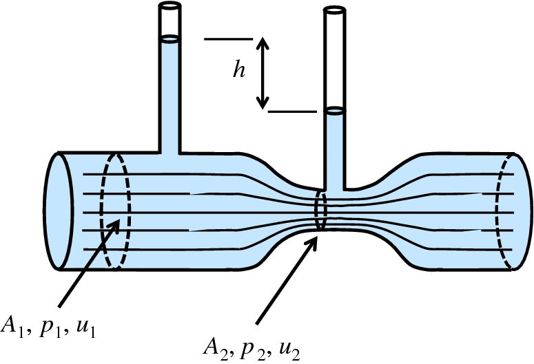
Figure 6.8 The principle of operation of a Venturi meter, which is used to measure fluid velocity in a pipe.

As we have seen, Bernoulli's equation is a statement of the conservation of energy. If gravitation forces are also involved, i.e. the fluid changes its vertical height, then we also include its gravitational potential energy, mgh, as for example in a hydroelectric power plant (see Section 7.1). (In the previous example, the change in height h was sufficiently small that we could neglect any change in gravitational potential energy.) Recalling that each term in Equation (6.10) represents energy per unit mass, we just need to add a term gh to Equation (6.10), We thus obtain:

(6.11)

This is the general form of Bernoulli's equation.

---

Worked example

Figure 6.9 shows a container of water with a small hole in its side that produces a jet of water. H is the depth of the container and h is the distance of the hole below the surface of the water. The jet of water strikes the floor at a distance x from the side of the container. (a) Determine x if H = 1.6 m and h = 0.40 m. (b) At what value of h should a second hole be drilled to give the same value of x? (c) What value of h gives the maximum value of x?

Solution

The size of the hole is small so that we can assume that the velocity at which the water level in the container falls is negligible. Also the pressure at the water surface and at the small hole are the same and equal to atmospheric pressure.

1. Taking the bottom of the container as the reference level for gravitational potential energy, we have from Bernoulli's equation
   
   where u is the velocity of the water jet. This gives . Interestingly, this is the same result for the final velocity of a body that falls under gravity through a distance h. The time, t, before the water jet strikes the ground is given by the expression:
   
   and hence . For the given values of H and h, x = 1.4 m.
2. Let height h' give the same value of x as h = 0.40 m. Then, using , we obtain:
   
   This simplifies to
   
   from which h' = 1.2 m or 0.40 m.
3. The distance x will be maximised when . This is when h = H/2, giving h = 0.80 m.

---

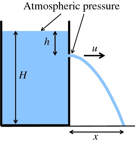
Figure 6.9 A container of water with a small hole in its side that produces a jet of water. H is the depth of the container and h is the distance of the hole below the surface of the water. The jet of water strikes the floor at a distance x from the side of the container.

Bernoulli's equation explains qualitatively the lift provided by an aeroplane wing. A section of a wing that moves through the air is shown in Figure 6.10(a). The streamlines crowd together above the wing corresponding to increased flow speed and reduced pressure, just as in the smaller diameter tube of the Venturi meter. Hence, the downward force due to the air on the top side of the wing is less than the upward force of the air on the underside of the wing, and there is a net upward or lift force, F_L. This force is perpendicular to the direction of the incoming air flow as shown in the figure.

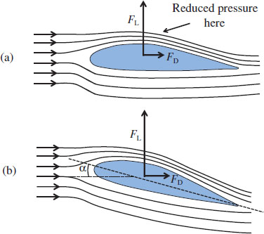
Figure 6.10 (a) When the air flows past an aeroplane wing, the streamlines crowd together above the wing, producing a lower pressure in that region. The upward force on the wing is then greater than the downward force on the wing and there is a net upward or lift force, F_L. The wing is also subject to a drag force F_D, which is due to frictional forces between the wing and the flow of air. (b) F_L can be increased by tilting the blade away from the incident wind direction within a certain range; the angle through which it is tilted is called the angle of attack, α. However, this also increases F_D.

In addition to the lift force, the wing is also subject to a drag force, F_D. The drag force is due to frictional forces between the wing and the flowing air. As illustrated in Figure 6.10(a), the drag force is parallel to the direction of incoming air flow. Both of these forces can be readily experienced by holding your arm out of a moving car and shaping your hand as the section of an aeroplane wing. The lift force, F_L, can be increased by tilting the blade away from the incident wind direction within a certain range, as in Figure 6.10(b). The angle through which it is tilted is called the angle of attack, α. However, this also increases the drag force F_D. We will see in Section 6.4 that the blades of a wind turbine experience the same forces as an aeroplane wing; the lift force and the drag force. In that case it is usually desirable to have the lift force to be as large as possible large compared with the drag force, as the drag force detracts from the desired action of the turbine. In a wind turbine, the angle of attack is controlled by twisting the blades about their long axis.

6.4 Extraction of wind power by a turbine

Before considering the extraction of wind power by a turbine, we consider the somewhat similar situation of a hosepipe directing a jet of water at a wall. A section of the hosepipe, which has uniform cross-sectional area A, is shown in Figure 6.11.

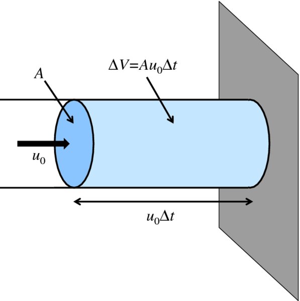
Figure 6.11 A section of a hosepipe with a uniform cross-sectional area A that carries water at velocity u₀ from left to right. In time Δt the volume of water that passes through area A is Au₀Δt.

Water travels through the pipe at velocity u₀ from left to right. In time Δt the volume ΔV of water that passes through area A is Au₀Δt. The mass Δm of this volume is ρAu₀Δt, where ρ is the water density and the momentum Δp is ρAu²₀Δt. Hence the rate at which momentum passes through area A, i.e. the momentum flow is given by

(6.12)

When the water eventually strikes the wall it exerts a force on the wall. Assuming that the water velocity reduces to zero at the wall, this force is then given by

(6.13)

The power P delivered to the wall is the rate at which the kinetic energy of the water is deposited at the wall. The volume ΔV of water has kinetic energy ΔK, which is given by

(6.14)

Hence,

(6.15)

Importantly, the delivered power P is proportional to the third power of the water velocity. Using (see Equation 6.6) we can also write the power as

(6.16)

We see that the flow of water exerts a force on the wall and delivers power to the wall. We can make a similar analysis for a wind turbine with air as the flowing fluid, as we will do below. However, there is a significant difference. The air that is incident upon the turbine cannot come to a sudden halt. It has to pass through the turbine in order for the blades to rotate and this must be taken into account. Albert Betz, a German physicist, obtained an expression for the maximum power, P_max, that can be extracted from the wind by a turbine. We can write his result as

(6.17)

where A_T is the area swept out by the turbine blades and u₀ is the wind speed. This equation is a statement of the Betz criterion. No matter what the design of the turbine or the shape of the blades, Equation (6.17) gives the maximum power that a turbine can extract from the wind. It has the same form as Equation (6.15) apart from the addition of the constant 0.59. In particular, the power is proportional to the third power of the wind speed. Of course, the density of air is much smaller than that of, water. However, this is compensated by the fact that commercial wind turbines sweep out a large area.

6.4.1 The Betz criterion

To obtain an expression for the Betz criterion, we consider a column of air of initial cross-sectional area A₀, as depicted on the left side of Figure 6.12. The initial wind speed is u₀. As the air approaches the turbine and passes through it, the wind speed reduces and hence, according to Equation (6.4), the cross-sectional area of the air column increases, as shown in (Figure 6.12). In this figure the area A_T represents the area swept out by the turbine blades, at which point the wind speed is u_T, which is less than u₀. We do not need to include the details of the turbine blades. We simply need to know that the wind exerts a force on them and that power is extracted from the wind. Finally, downstream of the turbine, the wind speed is reduced to u_f and the final cross-sectional area becomes A_f.

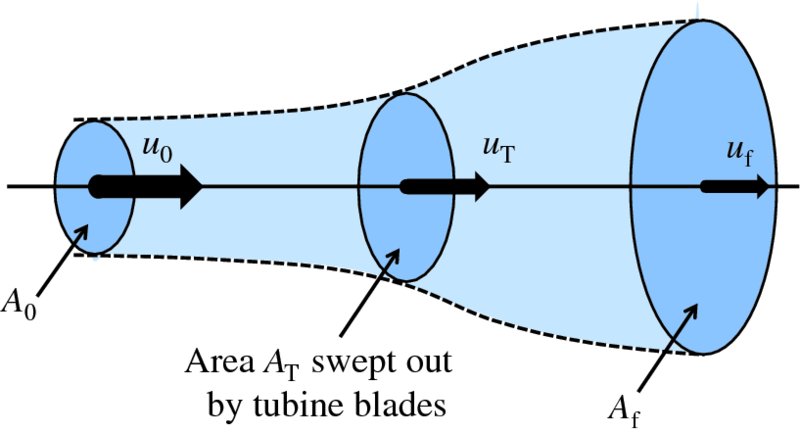
Figure 6.12 A column of air that is incident upon a wind turbine. The wind speed steadily decreases as the air approaches and passes through the turbine blades, which explains the evolution of the cross-sectional area of the air column. The area A_T represents the area swept out by the blades of the turbine. The wind exerts a force on the rotor blades and power is extracted from the wind.

In this process, the air mass flow through any cross-sectional area of the column is conserved and hence the mass flow at the three areas, A₀, A_T, and A_f, is the same:

(6.18)

We can find the power, P_T, extracted from the wind by considering the rate at which the wind loses its kinetic energy K. Recalling Equations (6.15) and (6.16) we have

Thus, at initial area A₀, the power in the wind is and at final area A_f it is . The power lost by the wind is equal to the power P_T extracted by the turbine, which is therefore given by

(6.19)

We can also find the power that is extracted from the wind by considering the change in momentum flow that the wind suffers in passing through the turbine. The momentum flow across initial area A₀ is, from Equations (6.12) and (6.6),

Similarly, the momentum flow across the final area A_f is

The difference between the initial and final momentum flow is just the force F acting on the turbine. Thus we have

(6.20)

We recall that mechanical work is force times distance and that power is the rate of doing work, i.e. force times velocity. Hence, the power P_T extracted by the turbine is given by

(6.21)

where u_T is the wind speed at the turbine. Equating Equations (6.19) and (6.21) we obtain

which gives

(6.22)

This result says that the wind speed at the turbine is the mean of the initial and final wind speeds. We have (see Equation 6.6), and substituting for in Equation (6.21) gives

(6.23)

Then using Equation (6.22) to eliminate u_f we obtain

(6.24)

We define the parameter a as the fractional decrease in wind speed:

(6.25)

giving

(6.26)

Substituting for u_T from Equation (6.26) into Equation (6.24) we obtain

(6.27)

The power P₀ in an unobstructed column of air of area A_T travelling with wind speed u₀ is given by

(6.28)

(see Equation 6.15). Thus the ratio P_T/P₀ = 4a(1 − a)² is a measure of the fraction of wind power extracted by a turbine and is called the power coefficient C_P. The power coefficient is plotted against a in Figure 6.13. The maximum value of C_P occurs when a = 1/3, when it has the value 0.59. From this value of a it follows from Equations (6.22) and (6.26) that for maximum power extraction the final wind speed u_f should be one-third of the initial wind speed u₀.

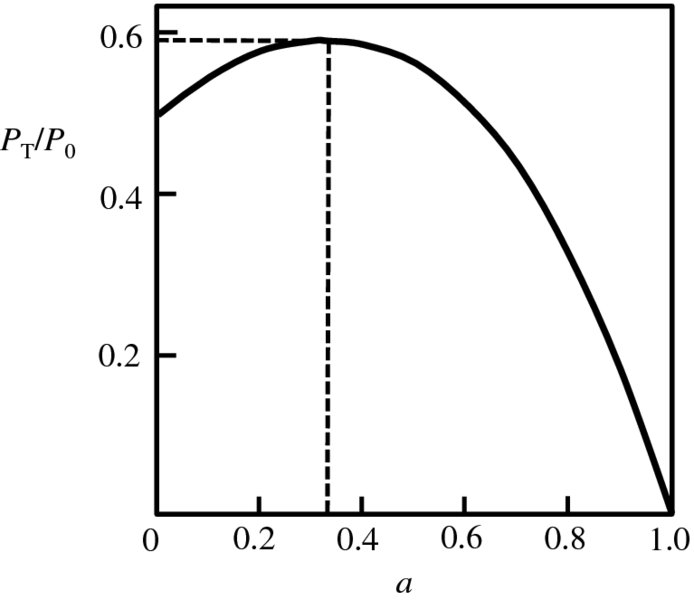
Figure 6.13 A plot of the ratio P_T/P₀ against a. This ratio is a measure of the fraction of wind power extracted by a turbine and is called the power coefficient. The parameter a is the fractional decrease in wind speed between the initial wind speed and the wind speed at the turbine blades. The maximum value of the power coefficient occurs when a =1/3, when it has the value 0.59.

In this analysis, we have assumed that the flow is laminar and there is no turbulence, i.e. that the air passes smoothly through the turbine. In practice, the motion of the turbine blades does produce some turbulence and, consequently, practical turbine efficiencies are less than the Betz limit. However, commercial wind turbines typically achieve 75–80% of the Betz limit. Note that the Betz limit has nothing to do with thermodynamic efficiency, but is instead a mechanical limit.

We can use Equation (6.28) to obtain a value for the typical power of unobstructed wind. Taking a wind speed u₀ = 10 m/s and an air density ρ = 1.2 kg/m³, we obtain a value for P₀ of 600 W/m². This is comparable to the power density of solar radiation at the surface of Earth.

---

Worked example

Estimate the number of wind turbines that would produce the same amount of power as a typical nuclear power station. Assume a blade length of 50 m and a wind speed of 10 m/s and that the turbine produces 80% of the Betz limit. Take the density of air to be 1.2 kg/m³.

Solution

The Betz criterion gives a value of P_max of

With a factor of 0.8 for overall efficiency, this reduces to 3.8 MW. Taking the output of a typical nuclear power station to be ∼1 GW, (see Section 3.4.5) this indicates that it takes ∼260 wind turbines to produce the same amount of power.

---

6.4.2 Action of wind turbine blades

The action of the blades of a wind turbine is to convert the linear motion of the incident wind into rotational motion of the rotor. Figure 6.14(a) shows one of the blades of a three-blade rotor as viewed from the front of the rotor. An element of the blade is indicated by the blue shaded area. It is at distance r from the axis of the rotor and rotates about it with angular velocity Ω and linear velocity u_lin = rΩ. Figure 6.14(b) shows the cross-section of this element as viewed from the blade tip and also indicates the plane of rotation of the blade. The turbine blade is similar in cross-section to the wing of an aeroplane (see Figure 6.10) and indeed the basic aerodynamics are the same for both. In the case of an aeroplane, the engines propel the wing through the air and a pressure difference develops between the top and bottom surfaces of the wing, thus producing a lift force, as we saw in Section 6.3. Similarly when the air flows across a turbine blade, a pressure difference develops between the two surfaces of the blade and a lift force is produced, as illustrated in Figure 6.14(b). The similarity between a turbine blade and an aeroplane wing can be seen by turning the page so that the direction of the incoming air flow in Figure 6.14(b) is horizontal. However, the blade is attached to the hub of the rotor and the net effect is that the blade rotates about the axis of the rotor.

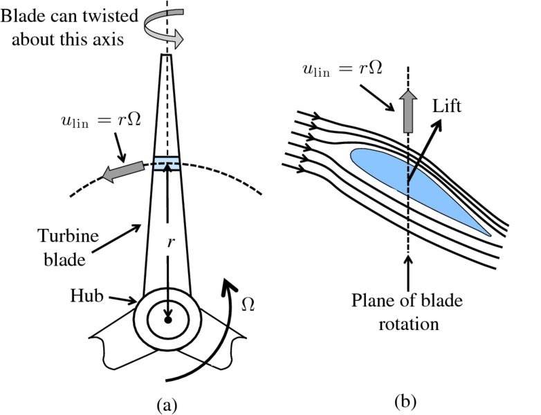
Figure 6.14 (a) One of the blades of a three-blade rotor as viewed from the front of the rotor. The blades rotate at angular velocity Ω in the plane that is perpendicular to the wind direction. An element of the blade at radial distance r from the rotor hub is indicated by the shaded area. It has linear velocity u_lin = rΩ. The blade can be twisted about its long axis to control the angle of attack. (b) The cross-section of the shaded element as viewed from the blade tip. When a wind flows across a turbine blade, a pressure difference develops between the two surfaces of the blade and a lifting force is produced. As the blade is attached to the hub of the rotor, the lifting force causes the blade to rotate about the axis of the rotor.

There is one particular difference between the action of a turbine blade and an aeroplane wing. The aeroplane wing experiences the wind coming directly towards it (see Figure 6.10). Similarly, a turbine blade experiences the incident wind with velocity u₀ coming directly towards the turbine. However, as the blade is rotating, it also experiences air coming towards it in its plane of rotation. This is called the rotational wind. The velocity of this rotational wind is just the linear velocity, u_lin = rΩ, of the blade. These two winds combine vectorially to produce the resultant or relative wind. It is the air flow due to the relative wind that is shown in Figure 6.14(b) and now we can see why its direction is not perpendicular to the blade's plane of rotation. The directions of the incident wind, the rotational wind and the relative wind with respect to the rotational plane of the rotor blades are illustrated in Figure 6.15. The velocities of these winds are u₀, u_rot and u_rel, respectively. Taking a value of u₀ of 12 m/s with r = 25 m, and a rotational frequency of the rotor of 15 rpm, we obtain u_lin/u₀ = (2π × 25)/(4 × 12) = 3.3. We see that the tips of the blades move much faster than the incident wind speed. This is because the blades experience the lift force.

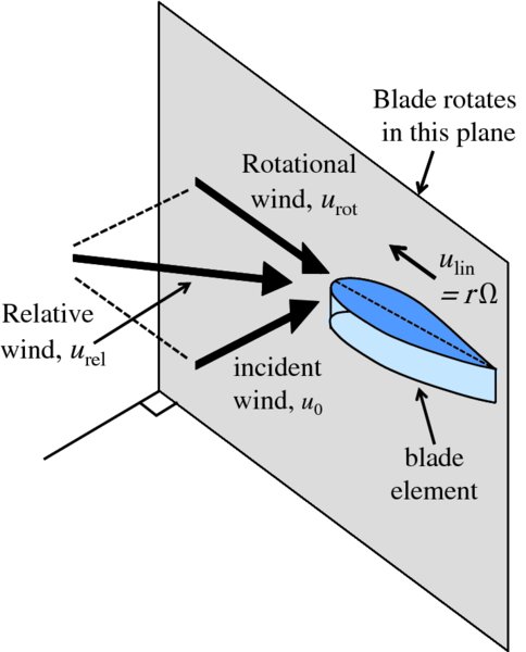
Figure 6.15 A turbine blade experiences the incident wind with velocity u₀ coming directly towards it. As the blade is rotating, it also experiences air moving towards it in its plane of rotation with velocity u_rot = u_lin = rΩ. These two winds combine vectorially to produce a resultant wind with velocity u_rel.

In most modern wind turbines, the angle of attack can be adjusted by changing the pitch of the blade, i.e. by twisting the blade about its long axis, as indicated in Figure 6.14. It is also the case that the optimum angle of attack depends on the ratio of the velocities u_rot/u₀ and clearly this ratio varies along the length of the turbine blade. This is taken into account by constructing the blade to have an inbuilt twist along its length.

Figure 6.16 illustrates the forces acting on an element of a turbine blade and the relevant wind velocities. The lift force, F_lift, and drag force, F_drag, combine to produce the total force, F_tot, acting on the element. This total force has a component F_pow in the plane of the rotation of the blades and it is this component that produces a torque on the rotor and hence the production of power by the turbine. The magnitude of F_pow, and hence the amount of power absorbed from the wind, is controlled by adjusting the angle of attack α, i.e. by adjusting the pitch of the blades.

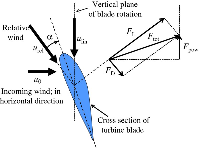
Figure 6.16 (a) The forces acting on a turbine blade are the lift force F_L and the drag force F_D. The lift force is perpendicular to the direction of the incoming air flow and is the consequence of the unequal pressure on the upper and lower surfaces of the blade. The drag force is parallel to the direction of incoming air flow, and is due to frictional forces between the wing and the flowing air. The lift force, F_lift, and drag force, F_drag, combine to produce the total force, F_tot, acting on the element. This total force has a component F_pow in the plane of the rotation of the blades and it is this component that produces a torque on the rotor and hence the production of power by the turbine. The magnitude of F_pow, and hence the amount of power absorbed from the wind, is controlled by adjusting the angle of attack α.

Commercial wind turbines that are used to generate electricity exploit the lift force F_L to turn the turbine rotor, as we have just described. But it is also possible to use the drag force F_D to cause a rotor to rotate. Indeed, the wind turbines that are seen, for example, on the plains of America exploit the drag force. Such turbines are recognisable by the many blades that their rotors have. They have characteristics that make them suitable for tasks such as pumping water from underground reserves.

Optimum rotational speed of turbine blades

The rotational speed of a wind turbine is very important in maximising its power output. If the rotational speed is too low, some wind will pass through without interacting with the blades. If it is too high, there will be excess wind turbulence, which decreases the efficiency of the turbine. In order to optimise the angular velocity of a rotor with respect to the incident wind speed, we compare the time t_b that it takes one rotor blade to move into the position occupied by the previous blade. If n is the number of blades and their angular velocity is Ω rads/s, t_b is given by

(6.29)

Suppose that the turbulence created by a turbine blade lasts time t_w. We need to wait at least that time before the following blade moves into its position. If d is the length of the wind that is perturbed by a rotating blade and u₀ is the wind speed,

(6.30)

It follows that for maximum power extraction we require t_b and t_w to be equal. This gives

or

(6.31)

where R is the radius of the blades. Defining the tip-speed ratio λ as

(6.32)

there is maximum power extraction when λ = 2πR/nd. Experimental measurements show that d ≈ R/2, and hence λ ≈ 4π/n. This suggests that a three-blade rotor, say, has an optimum tip-speed ratio of ∼4. By designing turbine blades with highly aerodynamic efficiency, the effects of turbulence can be minimised and this can increase the value of the tip-speed ratio to about 6 or 7. This leads to higher rotational speeds of the rotor and hence higher power output. Tip-speed ratio is probably the most important parameter of a wind turbine, as it is a function of the three most important variables: blade radius R, wind speed u₀ and rotor angular velocity Ω. Being dimensionless, it is an essential scaling factor in wind turbine design.

6.5 Wind turbine design and operation

There are various types of wind turbine. These can be divided into those that rotate about a horizontal axis and those that rotate about a vertical axis. The horizontal axis type is the most common today and is our primary focus. These typically have three blades, as illustrated in Figure 6.17(a). Turbines that rotate about a vertical axis are exemplified by the Darrieus turbine, which is illustrated in Figure 6.17(b). Vertical axis turbines have some advantages. They work in any wind direction. Moreover, as their axis of rotation is vertical, they do not suffer from the gravity-induced stress/strain cycles that occur in a horizontal axis turbine when the blades rotate. Disadvantages of a vertical axis turbine are that their overall efficiencies are generally less than for horizontal axis turbines and they not self-starting; they must be given an impulse to start rotating.

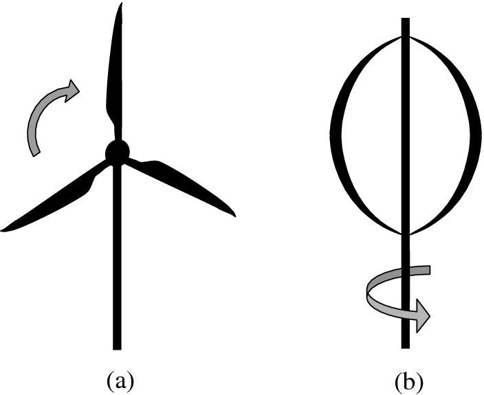
Figure 6.17 (a) The horizontal axis wind turbine is the most common type today and typically has three blades. (b) The Darrieus wind turbine exemplifies those types that rotate about a vertical axis.

The main components of a horizontal axis wind turbine are shown in Figure 6.18. These include the rotor, the gearbox and the electrical generator. The rotor consists of the turbine blades and a supporting hub that connects the blades to the main shaft of the turbine. The blades are typically made from composites, primarily fibreglass or plastics reinforced with carbon fibres. As noted previously, in modern turbines, the pitch of the blades can be varied to control the power output from the turbine. The housing that contains the mechanical and electrical components of the turbine and protects them from the weather is called the nacelle. The whole assembly is mounted on a support tower. The rotor may be in front (upwind) of the support tower or behind it (downwind). Wind veers frequently in direction and horizontal axis turbines must be turned into the wind for maximum power output. Downwind turbines are, in principle, self-orientating. However, the rotor is then in the shadow of the tower, and this produces extra turbulence. Moreover, as the rotor rotates, there will be times during the cycle when one of the blades falls within the wind shadow and this leads to uneven loading across the rotor and mechanical stress. Upwind turbines, as in Figure 6.18, avoid these disadvantages but they must be driven to face the incident wind. This is done under computer control by the yaw mechanism, which consists of a large bearing that connects the body of the turbine to its support tower; this mechanism gets its control signal from a wind direction sensor mounted on the nacelle. Most commercial wind turbines are of the upwind variety. Wind turbines also incorporate a brake that can be engaged to close down the turbine for maintenance or for when the wind speed is so high that it could damage the turbine.

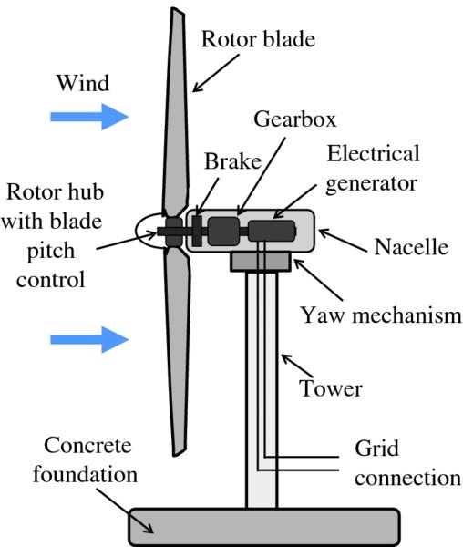
Figure 6.18 The main components of a horizontal axis wind turbine. These include the rotor, the gearbox and the electrical generator. The rotor consists of the turbine blades and a supporting hub that connects the blades to the main shaft of the turbine. The housing that contains the mechanical and electrical components of the turbine and protects them from the weather is called the nacelle. The whole assembly is mounted on a support tower. The yaw mechanism consists of a large bearing that connects the body of the turbine to its support tower and is used to turn the turbine into the wind. The purpose of the gearbox is to match the rate of rotation of the rotor (5–20 rpm) to that of the generator (∼1000 rpm). Wind turbines also incorporate a brake that can be engaged to close down the turbine for maintenance or for when the wind speed is so high that it could damage the turbine.

Most commercial wind turbines have three blades. This number, like many design considerations, is a compromise between competing requirements. These include aerodynamic efficiency, mechanical stability, manufacturing cost, and environmental and aesthetic issues. The aerodynamic efficiency of a rotor does increase with the number of blades but with diminishing returns. For example, the improvement in going from two to three blades is ∼5% and in going from three to four blades is ∼1%. As the number of blades increases, the balance and hence the stability of the rotor increases, which means less mechanical stress on the turbine as it rotates. Thus the lack of balance in a one-blade rotor can cause can cause high levels of mechanical stress in the rotor, even though the blade is balanced by a counterweight. Twin-blade rotors are better balanced. However, yawing operations, where the nacelle and rotor turn around a vertical axis, have to take place slowly to limit fluctuating dynamic loads during the operation; when the blades are vertical the forces required to yaw the rotor are low, but when the blades are horizontal, the forces are much higher. These cyclic forces impose significant stresses on the turbine. Three-blade rotors are more balanced than one- or two-blade rotors. Moreover, the fluctuating dynamic loads are much lower when a three-blade machine is yawed, as the asymmetric forces encountered as the rotor rotates are smaller. Four-blade rotors are better balanced still. There are, however, some drawbacks that arise with an increase in the number of blades. As the number of blades increases, so too do the manufacturing costs. Moreover, the solidity of a rotor must be kept to a reasonably low value, where solidity is the ratio of the total area of the blades and the area swept out by the blades. Thus, as the number of blades increases, they must be thinner. And then it becomes difficult to build blades that are sufficiently strong and more expensive materials are required. Taking all considerations into account, three-blade turbines appear to provide the best compromise, as evidenced by the fact that most commercial turbines have three blades, and it is generally accepted that three-bladed turbines are less noisy and less visually disturbing than other possible designs.

The rotor of a wind turbine usually rotates within the range 5–20 rpm. On the other hand, the drive shaft of a conventional electrical generator rotates at ∼1000 rpm. The purpose of the gearbox is to match the rotational speeds of the rotor and the generator. A typical gearing ratio is 1:50. On large wind turbines, the generated electricity is usually 690 V three-phase AC.

A wind turbine may be designed to operate at fixed rotor speed, i.e. at fixed angular velocity or with variable rotor speed. Most commercial wind turbines are connected, via a transformer, to a national electricity grid. As these operate at a fixed frequency, usually 50 or 60 Hz, it follows that the electrical generator must also operate at a constant or nearly constant frequency. In a fixed-speed turbine, this determines the angular velocity, Ω, of the rotor. The disadvantage of this fixed-speed mode of operation is that the optimum tip speed ratio:

is not maintained if Ω is kept constant but wind speed u₀ changes, although in practice the reduction in overall efficiency is usually not substantial. Most modern turbines have variable-speed operation. This has the advantage that the tip-speed ratio can be kept constant at its optimum value over a wide range of wind speeds, thus operating the turbine at maximum efficiency. However, the varying speed of the rotor clearly complicates the generation of AC electricity at constant frequency. There are a variety of ways to allow variable-speed operation of the turbine rotor while keeping the generating frequency constant. These may be mechanical or electrical, although most approaches to variable-speed operation in use today are electrical in nature. These involve solid-state power convertors, which can change electrical power from one frequency to another.

The operating regions for a wind turbine are illustrated by the example of a wind power curve shown in Figure 6.19. At very low wind speeds, there is insufficient torque exerted on the turbine blades to make them rotate. However, as the speed increases, the turbine begins to rotate and to generate electrical power. The minimum speed at which the turbine blades overcome friction and start to rotate is called the cut-in speed and is typically between 3 and 4 m/s. As the wind speed rises above the cut-in speed, the output power rises rapidly; we recall that the power in the wind increases as the third power of its speed. The range in which the turbine produces output power is indicated by the blue shaded area in Figure 6.19. When the wind speed becomes greater than ∼14 m/s, the absorbed wind power is limited to a constant value to avoid exceeding safe electrical and mechanical loading limits. This limit is called the rated power output and the speed at which it is reached is called the rated output speed. In large turbines, the power is typically limited by controlling the pitch of the rotor blades. As the wind speed increases above the rated output wind speed, the forces on the turbine structure continue to rise and, at some point, there is a risk of damage to the rotor. As a result, the braking system is employed to bring the rotor to a standstill. This is called the cut-out speed and is usually ∼25 m/s.

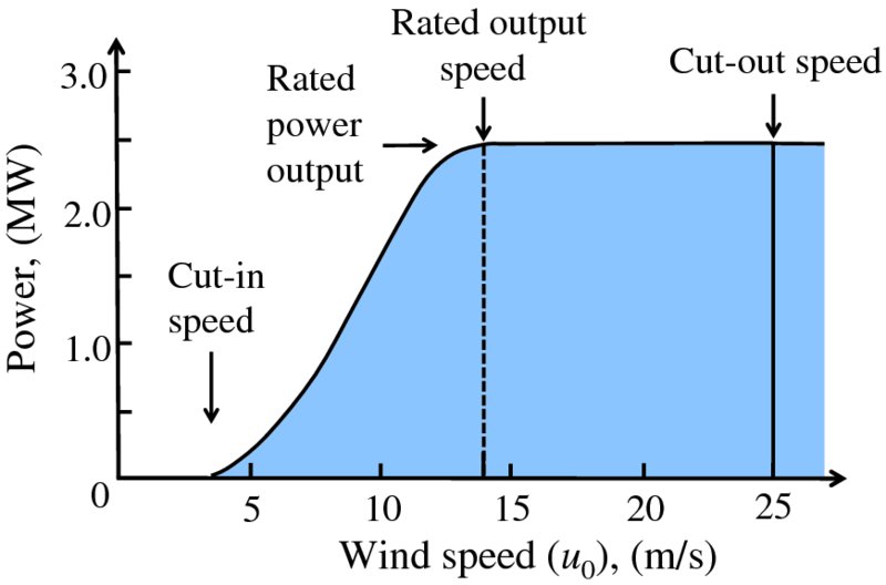
Figure 6.19 The operating regions of a wind turbine. At very low wind speeds, there is insufficient torque exerted on the turbine blades to make them rotate. However, as the speed increases, the turbine begins to rotate and to generate electrical power. The minimum speed at which the turbine blades rotate is called the cut-in speed. As the wind speed rises, the output power rises rapidly; the blue shaded area in the figure is where the turbine produces output power. When the wind speed becomes greater than ∼ 14 m/s, the absorbed wind power is limited to a constant value to avoid exceeding safe electrical and mechanical loading limits. This limit is called the rated power output and the speed at which it is reached is called the rated output speed. At wind speeds above the cut-out speed, the turbine rotor is stopped from turning to avoid excessive operating loads.

Typical values for a commercial wind turbine that is connected to a national grid are as follows: a rotor diameter of ∼100 m; a hub height of ∼80 m; an operational range of wind speed of 4–25 m/s; and a nominal output power of 3.6 MW. This is sufficient for more than 3000 average households. Currently, the largest wind turbines have a rated capacity of 8 MW and a rotor diameter of 164 m.

A possible electrical arrangement for a variable-speed wind turbine that is located in a remote region and not connected to a national grid is shown schematically in Figure 6.20. The generator produces an AC voltage of variable frequency and variable amplitude. Some electrical loads, such as resistive elements to heat water, do not need constant AC frequency or supply voltage and so the output from the generator can be applied directly to them. Applications that are sensitive to frequency and amplitude can be supplied by a separate voltage line, as outlined in Figure 6.20. The AC voltage from the generator is converted to a smoothed DC voltage by a diode bridge/capacitor circuit. This voltage is then regulated in amplitude and the regulated voltage is connected to a battery that provides energy storage. This regulated voltage also drives an oscillator that operates at the required frequency, say 50 Hz. Typically the oscillator gives an output waveform that is not a pure sine wave; it may give a square waveform as shown in the figure. The square waves can, however, be converted into a waveform that is closer in shape to a sine wave by a low-pass filter. This filter consists of a combination of inductances and capacitors that reduce the harmonics of the square wave that lie above the fundamental frequency. The filtered voltage is applied to a transformer that raises the voltage amplitude to the required value, say 240 V.

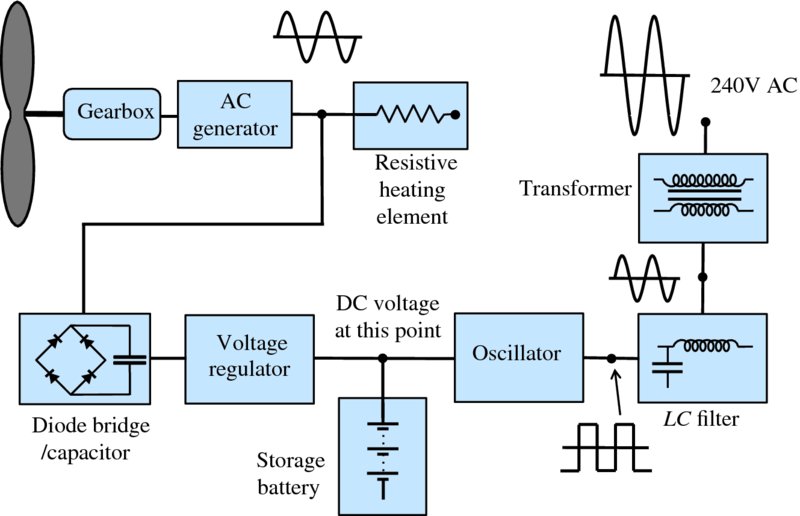
Figure 6.20 A possible electrical arrangement for a variable-speed wind turbine that is not connected to a national grid. This arrangement provides electrical power for applications, such as resistive elements to heat water that do not need constant AC frequency or supply voltage. It also provides a separate 240 V, 50 Hz AC voltage line for applications that are sensitive to frequency and amplitude.

---

Worked example

Figure 6.21(a) illustrates a simple version of an alternator that converts mechanical energy to electrical energy in the form of alternating current. The wire loop of area A rotates with constant angular frequency ω about the axis shown. The magnetic field B is uniform and constant. Obtain an expression for the induced emf ϵ as a function of time t. At time t = 0, θ = 0.

Solution

When the loop makes angle θ with respect to the direction of the magnetic field B, the magnetic flux ϕ through the loop is ϕ = BAcos θ (see Figure 6.21b). Hence by Faraday's law (Equation 6.1), the induced emf is

Figure 6.22(a) shows the variation of ϵ with time and also the variation of magnetic flux through the loop. Figure 6.22(b) shows the corresponding orientations of the coil. The physical principle outlined in this example is the basis for the operation of electrical generators, in this case for an AC current generator.

---

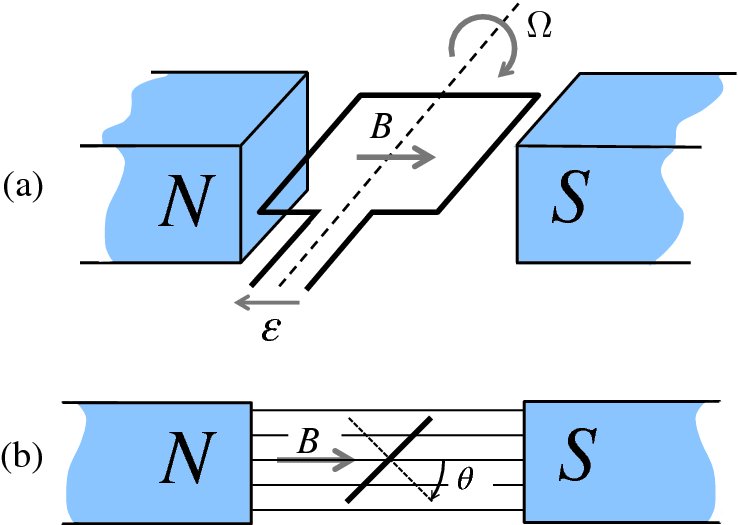
Figure 6.21 (a) A simple version of an alternator that converts mechanical energy to electrical energy in the form of alternating current. The wire loop of area A rotates with constant angular frequency ω about the axis shown. The magnetic field B is uniform and constant. (b) Side view of the alternator.

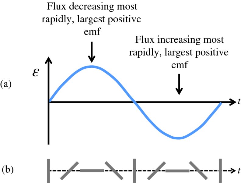
Figure 6.22 (a) The variation of the induced emf, ϵ, with time for the alternator in Figure 6.22; (b) the corresponding orientations of the loop.

6.6 Siting of a wind turbine

The siting of a wind turbine is of paramount importance in maximizing the amount and speed of the wind it receives. We recall that the power harvested by a wind turbine varies rapidly as the third power of the wind speed and, in practice, the wind must have a minimum average speed of ∼5 m/s for a turbine to function effectively. Factors that influence turbine siting include: (i) the directions of prevailing and local winds; (ii) the local terrain such as hills and mountains; (iii) any local obstacles such as houses and trees; (iv) environmental issues such as noise and visual impact; and (v) what is called the roughness of the terrain. For example, a water surface or a flat, open landscape that is grazed by sheep has a low degree of roughness. On the other hand, long grass and shrubs have a high degree of roughness. In general, the more pronounced the roughness of the terrain, the more the wind will be slowed down. Offshore wind turbines benefit from the fact that the roughness of the water surface is usually low and obstacles are few.

Within the height of local obstacles, wind direction changes erratically and there may be large-scale fluctuations in wind speed. Above this erratic region the wind speed u(z) is found to vary logarithmically with vertical height z, with the form

(6.33)

In this expression, V is a characteristic wind speed, d is roughly equal to the height of local obstacles and z₀ is a length that characterizes the roughness of the terrain. For rough pasture z₀ may be ∼10 mm, while for forest and woodlands it may be ∼500 mm. Figure 6.23 is a sketch of the variation of u(z) with z, together with typical values of wind speed. Clearly, the taller the turbine, the higher the wind speed. However, because of the logarithmic dependence of u(z) on height, it is considered that there is not much to be gained above a height of about 100 m. Notice from this figure that the wind speed varies across the area swept out by the rotor blades and this causes forces across the turbine that must be taken into account in the design and construction of the turbine.

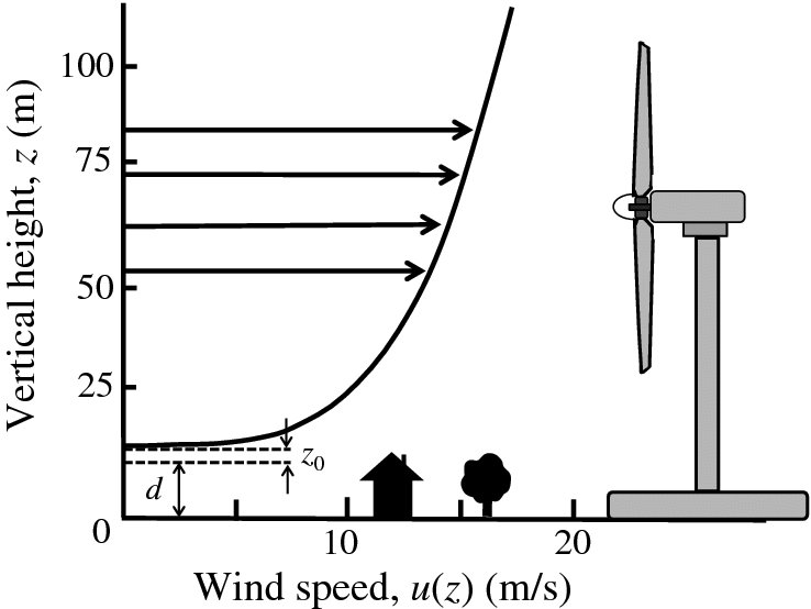
Figure 6.23 Variation of wind speed, u(z), with vertical height, z. Within the height of local obstacles, wind direction changes erratically and there may be large-scale fluctuations in wind speed. Above this erratic region, u(z) is found to vary logarithmically with vertical height.

A wind farm consists of many wind turbines and indeed a large wind farm may consist of several hundred individual turbines. The Alta Wind Energy Centre (Mojave Wind Farm) in California, USA, is the largest onshore wind farm outside China, and will see the installation of 600 wind turbines supplying 1.5 GW of power. The London Array is a 175-turbine offshore wind farm located 20 km off the Kent coast in the UK and delivers 630 MW of power. It is the largest offshore wind farm in the world, and the largest wind farm in Europe by megawatt capacity (see Figure 6.24).

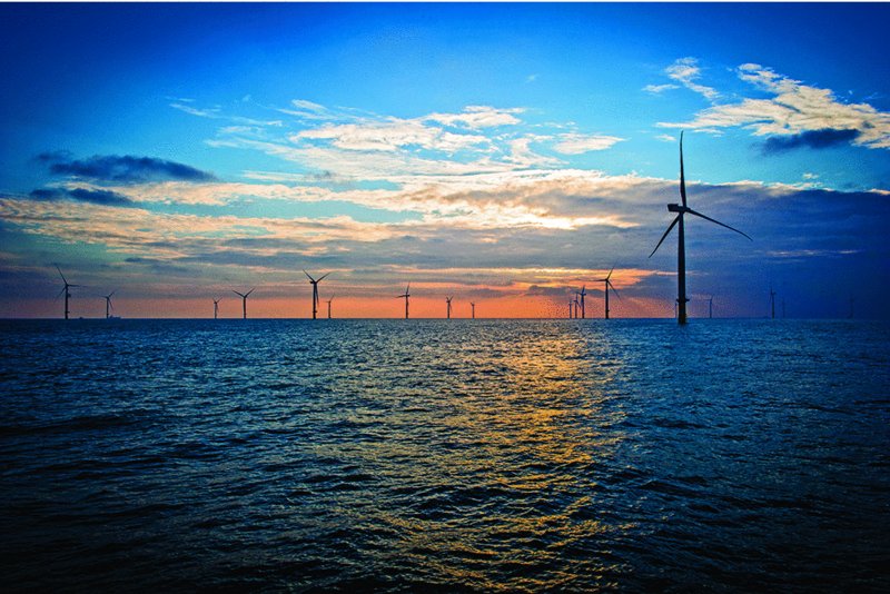
Figure 6.24 The London Array offshore wind farm located 20 km off the UK's Kent coast. The London Array has 175 turbines and delivers 630 MW of power. It is the largest wind farm in Europe by megawatt capacity. Courtesy of London Array Limited. http://www.londonarray.com/offshore-2/

A wind turbine produces wind turbulence downstream of the turbine and so individual turbines in a wind farm must be separated by at least five times the rotor diameter, D, to reduce the effects of this turbulence. Figure 6.25 is a schematic diagram of adjacent turbines in a wind farm, separated by five rotor diameters. We see that the area allocated to an individual turbine is proportional to D². However, we recall that the power extracted from the wind by a turbine is proportional to the area swept out by the rotor blades, which is also proportional to D² (Equation 6.28). Hence we have the important result that the power per unit area of a wind farm is independent of rotor diameter. It does, however, depend on wind speed. For wind speeds that are obtained in practice, the extracted wind power per unit area of wind farm lies within the range of approximately 1–10 W/m².

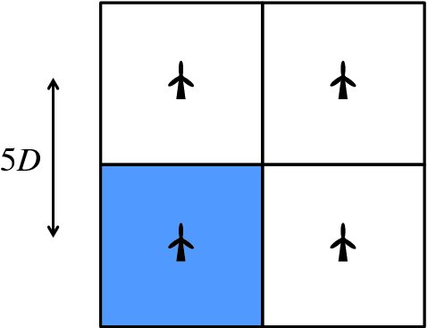
Figure 6.25 A schematic diagram of adjacent turbines in a wind farm that are separated by 5D, where D is the rotor diameter.

A particularly effective site for a wind turbine is on top of a hill overlooking the surrounding countryside. This gives a wide view of the prevailing wind. In addition the wind speed will increases toward the top of the hill. This effect is illustrated in Figure 6.26. The wind becomes compressed on the hillside facing the prevailing wind direction as it reaches the top of the hill, just as a fluid does in the narrow bore of a Venturi meter. This, in turn, increases the wind speed at the top of the hill.

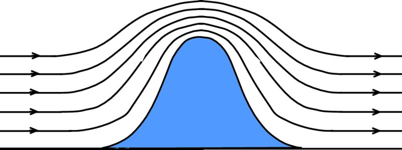
Figure 6.26 A particularly effective site for a wind turbine is on top of a hill overlooking the surrounding countryside. This gives a wide view of the prevailing wind. In addition, the wind speed will increase towards the top of the hill. The wind becomes compressed on the hillside facing the prevailing wind direction as it reaches the top of the hill. This in turn increases the wind speed.

Problems 6

1. Each blade of a wind turbine has a length of 35 m. If the wind speed is 15 m/s and the density of the air is 1.1 kg/m³, calculate the power generated by the turbine if it achieves 75% of the Betz criterion. What power would be generated if: (i) the density of the air is 20% higher; (ii) the blades were 20% longer; and (iii) the wind speed is 20% higher?

2. A ball is thrown with uniform velocity v from the centre of a platform that rotates in a counter-clockwise direction at angular velocity Ω. To an observer at the centre of the platform, the ball appears to move towards the right. Show that the ball appears to move to the right with acceleration 2vΩ.

3. 

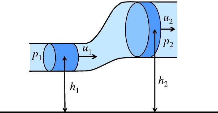
    (a) The flow of a liquid through a pipe that has varying bore and height is illustrated in the figure. Use conservation of energy to show that

   

   where the symbols have their usual meanings. (b) Water is supplied to a house through an inlet pipe with an internal diameter of 40 mm. A pipe of internal diameter 20 mm delivers water to a bathroom 5.5 m above the inlet pipe at the rate of 4 L/min and at the pressure of 2 atm. Calculate the required pressure at the inlet pipe to the house? Take 1 atm = 1 × 10⁵ Pa.

4. Suppose the difference between the velocity u_t at the top of an aeroplane wing and the velocity u_b at the bottom of the wing can be written as (u_t − u_b) = ku₀, where u₀ is the velocity at which air approaches the wing and k is a constant characteristic of the wing shape and the angle of attack. Show that the lift force on the aeroplane is given by F_L = Aρku²₀, to a good approximation when k ≪ 1, where A is the total area of the wings and ρ is the air density. If the mass of the aeroplane is 3000 kg, A = 40 m², ρ = 1.2 kg/m³ and k = 0.1, what is the value of u₀ when the lift force balances the force of gravity?

5. The power coefficient C_P is given by C_P = 4a(1 − a)². Show that the maximum value of C_P is 0.59 when a = 1/3.

6. Show that the force per unit area F_A ( = F_T/A_T) acting on a turbine is given by

   

   where the symbols have their usual meanings. At what value of a is F_A a maximum? Calculate the maximum value of F_A for an incident wind speed of 20 m/s. In this case, what is the value of the final wind speed u_f? Compare the maximum value of F_A with the value of F_A when a = 1/3. Take the density of air to be 1.2 kg/m³.

7. (a) A wind turbine is maintained at a tip-speed ratio of 6 for all wind speeds. At what wind speed would the blade tip speed be equal to the speed of sound? (b) An offshore wind turbine has a rotor diameter of 100 m. At what frequency (Hz) of the rotor would the tip speed be equal to the speed of sound? Why should operation at a tip speed exceeding the speed of sound be prevented?

8. (a) Assuming that the turbines in a wind farm need to be five rotor diameters apart, as in Figure 6.25, calculate the power that can be extracted from the wind per square metre of the wind farm at a wind speed of 8 m/s. Assume that the turbines achieve 80% of the Betz criterion and that the density of air is 1.2 kg/m³. (b) Using your estimate from part (a), estimate the total area of a wind farm that would generate the same power as a typical nuclear power station.

9. The power P in an unobstructed column of air of area A travelling with wind speed u is given by . An approximate expression that is often used to determine wind speed u_z at height z is u_z = u_s(z/h₀)^0.14m/s, where u_s is the speed at z = 10 m and h₀ = 10 m. Make a plot of wind power per unit area (P_z/A) in units of (P_s/A) against height z over the range of z from 10 to 250 m, where P_s is the wind power at z = 10 m. Comment on the use of turbines with small rotor diameters, say 5 m, above 100 m.

10. A conducting disk with radius R rotates about its central axis with constant angular frequency ω in a uniform magnetic field B. Show that the emf between the centre and rim of the disk is given by