7
Water power
Earth has a huge amount of water – it covers about three-quarters of the planet. Interestingly, scientists are not sure how and when it got here. One theory is that the water was brought by meteorites or asteroids, both of which contain ice. We derive mechanical power from this water in various ways. This includes hydroelectric power, ocean wave power and tidal power. Water power has been exploited by mankind for thousands of years. For example, the Doomsday Book (AD 1065) records that there were more than 5000 water mills in operation in England at that time. Their main use was to grind corn into flour. Much later, water mills powered the first period of the Industrial Revolution. And although water power later gave way to steam power, it still found use for small-scale operations during the 18th and 19th centuries. In contemporary times, water power has again become significant as it provides a clean, renewable and potentially cheap energy source. In particular, hydroelectric power is now well established. Indeed, in some countries, like Norway and Brazil, hydroelectric power is the dominant source of electricity. Ocean waves and tides are relative newcomers as commercial energy sources and as yet do not provide substantial contributions to world energy demands. This is despite the fact that many hundreds of patents have been taken out on ways of harnessing wave and tidal power.
Hydroelectric power, wave power and tidal power form the three main sections of this chapter. In each case we will describe the main physical principles involved and how the energy is harnessed. This will involve a discussion of the nature of wave motion and the origin of the tides.
7.1 Hydroelectric power
Hydroelectric power is by far the most established and widely used renewable energy source for electricity generation and accounts for ∼20% of the world's electricity supply. By hydroelectric power, we mean power that is obtained from water that falls through a vertical distance from a reservoir to drive a turbine. This is in contrast to, say, water mills, which draw power from a flowing river. Hydroelectric power has important advantages. Once constructed, hydroelectric plants produce minimal pollution with considerably lower output levels of greenhouse gases than fossil fuel plants. They also have the potential to produce energy at low cost because once it is built, a hydroelectric plant will run for many years with just routine maintenance. The potential energy of the stored water in a reservoir also provides a natural store of energy that can be used to even out variations in seasonal rainfall and varying electricity demand. (In an analogous way, the large ∼5000 μF electrical capacitor in the power supply of a domestic audio amplifier evens out the variation in the voltage supplied by the diodes that rectify the mains voltage, and the varying current demands of the amplifier. Not surprisingly, it is called a reservoir capacitor.) The stored energy in the reservoir of a hydroelectric plant is readily available as a turbine/electrical generator combination can be switched on within minutes to meet additional demand. Consequently, hydroelectric power can be used to supply both base load and peak demand on a national grid supply. This ability of a hydroelectric plant to store energy is taken a step further in pumped storage, which we describe in Section 8.4.1. Briefly, water is pumped back into the reservoir from a reservoir that is at a lower height when electricity demand is low, say during the night or at the weekend. Then, when demand increases at peak times, water is released back into the lower reservoir through a turbine.
The main disadvantages of hydroelectric power lie in its impact on the local environment. This includes social impact if there is a displacement of people from the reservoir site, loss of potentially productive land and disruption to surrounding aquatic ecosystems, both upstream and downstream of the plant. In addition, hydroelectric plants have relatively large constructional costs, although once established the cost of hydroelectricity is relatively low, as noted earlier.
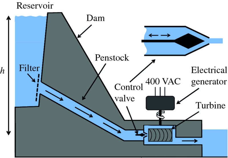
Figure 7.1 A schematic diagram of a hydroelectric plant. The water reservoir is connected to a turbine by a large pipe called a penstock. The filter keeps debris from entering the turbine, while the valve controls the water flow and hence the rotational speed of the turbine and the electrical generator. The vertical distance h between the surface of the water in the reservoir and the turbine is called the head. The turbine drives a generator that produces electrical power at an output voltage of typically 400 VAC.
7.1.1 The hydroelectric plant and its principles of operation
A schematic diagram of a hydroelectric plant is shown in Figure 7.1. There is a reservoir that collects rainwater from a large catchment area. Often the reservoir is formed from a naturally occurring geographical feature to which a dam is added to confine the water. A large pipe, called the penstock, delivers the water to a turbine. The vertical distance between the surface of the water in the reservoir and the turbine is called the head. A filter at the input of the penstock stops any debris from entering the turbine. There is also a valve at the output of the penstock that is used to control the flow of water delivered to the turbine and hence its rotational speed. The turbine drives a generator that produces electrical power at an output voltage of typically 400 VAC. This is fed to a step-up transformer (not shown), which converts the voltage to a higher value that is suitable for long-distance transmission. The ability to transport electricity over long distances is very useful in this case as hydroelectric plants are usually remote from urban centres. Although the electricity from a hydroelectric plant is usually delivered to a national grid in this way, some plants are used exclusively for a nearby manufacturing process. A good example is the electrolytic production of aluminium, which requires a lot of electrical power. For large hydroelectric plants like the Itaipu Dam, which is located on the border of Brazil and Paraguay, the output power can be large, greater than 10 GW. (The Itaipu Dam was elected as one of the seven modern wonders of the world by the American Society of Civil Engineers.) But there are also smaller plants producing ∼10 MW and even micro plants that deliver ∼5–100 kW, which are suitable for small communities.
It is important to note that there is no intermediate thermal process involved in hydroelectric power. The falling water drives a turbine directly. This is in contrast, for example, to a nuclear power plant where there is an intermediate thermal step in which the nuclear energy is first used to produce steam which then drives a turbine. Hence for a hydroelectric plant there is no fundamental thermodynamic limit to the conversion of water power into mechanical power. We can make the same comment about wind turbines, which again drive an electrical generator directly.
The principle of hydroelectric power is straightforward. Water falls a certain vertical distance and its potential energy is transformed into kinetic energy. This kinetic energy is then converted into mechanical energy by the turbine. Suppose that a volume per second, Q, of water falls a vertical distance h. Then the mass of water falling per second is ρQ, where ρ is the density. Then the rate of potential energy lost by the falling water, i.e. the power P, is given by
where g is the acceleration due to gravity. This is the fundamental equation for hydroelectric power. Clearly, the larger the flow rate Q and the larger the vertical distance h, the greater the power that is obtained. This result assumes that there are no losses due to friction. In a hydroelectric plant, however, there is friction between the flowing water and the internal surface of the penstock. Thus the actual power that can be obtained from the falling water is less than that given by Equation (7.1), as we describe in the following section.
7.1.2 Flow of a viscous fluid in a pipe
Viscosity is the internal friction in a fluid. All real fluids have viscosity. Some, like water, have relatively low viscosity, while other fluids, such as maple syrup, have relatively high viscosity. We saw in our discussion of wind turbines that air is also a fluid and it, too, has viscosity. The viscosity of air, however, is about 50 times less than that of water. The frictional forces due to viscosity oppose the motion of one portion of the fluid relative to another. These frictional forces are significant and, indeed, the flow of a viscous fluid in a pipe is one of the most important problems in fluid dynamics. They arise, for example, in the circulation of blood in the human body.
The effect of viscosity is to reduce the fluid pressure as the fluid travels through a pipe. For example, it is common experience that the water pressure at the outlet of a hosepipe is lower than the water pressure at the tap; the longer the pipe the greater the loss in pressure. Figure 7.2 illustrates the flow of a viscous fluid in a pipe. It shows the velocity profile of the fluid, where the horizontal arrows indicate the magnitude of the fluid velocity at various values of radial distance r. Due to its viscosity, the velocity of the fluid in immediate contact with the walls of the pipe is zero, while the velocity is greatest at the centre of the pipe. The motion of the fluid is rather like a set of concentric tubes sliding relative to each other – the tube at the centre of the pipe moves fastest and the outermost tube is at rest. The viscous forces oppose the sliding of the tubes. The result is that the velocity profile of the fluid is parabolic in shape, as shown in Figure 7.2.
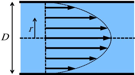
Figure 7.2 The figure represents the flow of a viscous fluid in a pipe of internal diameter D. The horizontal arrows represent the magnitude of the velocity of the fluid at various values of radial distance r. The velocity of the fluid is zero at the walls of the pipe due to frictional forces and reaches a maximum at the centre of the pipe. The motion of the fluid is rather like a set of concentric tubes sliding relative to each other; the tube at the centre of the pipe moves fastest and the outermost tube is at rest. The viscous forces oppose the sliding of the tubes. The result is that the velocity profile of the fluid is parabolic in shape.
Away from the ends of a pipe, the pressure drop per unit length is constant. Thus, neglecting the end effects, we may say that the pressure drop, Δp, along the pipe is linearly proportional to its length L, i.e. Δp∝L. It is useful to scale the pipe length in terms of the pipe diameter D. We can then write
The friction increases with fluid velocity u, just as it does for a sphere dropping through a viscous fluid, as described by Stokes’ law. Hence, Δp also increases with fluid velocity. From Bernoulli's equation,
we see that the quantity
 has the same dimensions as p. All of these characteristics can be expressed in a single equation:
This is not a derivation of this important equation. However, it does illustrate the significant physical quantities involved and it also hints at the use of dimensional analysis in its derivation.
Dimensional analysis is widely employed in fluid mechanics, where the complexity of the situation means that it is not possible to solve the problem from first principles. Indeed, the technique is used in many fields of engineering for the same reason. A familiar example of the use of dimensional analysis is to obtain an expression for the period of a simple pendulum. If we say that the period T depends on the length l of the pendulum, the mass m of the pendulum and the acceleration due to gravity g, we have
From the dimensions of these physical quantities we have
Then equating coefficients of the exponents we find:

Thus we obtain
 , as expected. Of course the dimensional analysis does not give the constant of proportionality.
We now return to Equation (7.3) and recall the general expression p = ρgh, where p is the pressure due to a column of fluid of height h. Thus we can express the drop in pressure, Δp, due to friction in terms of a quantity called the head loss, hf:

giving
The constant of proportionality, fD, is a dimensionless constant that incorporates the fluid viscosity. It is called the Darcy friction factor, named after French engineer Henry Darcy and this equation is called the Darcy–Weisbach equation. The value of fD for a given pipe can be obtained from empirical or theoretical relationships or from published tables.
We interpret the head loss hf as the loss in vertical height due to frictional forces. Thus instead of using the actual head, i.e. vertical height h in Equation (7.1), we use instead the available head, ha, where
The value of hf depends linearly on the length of the penstock, which connects the water reservoir to the turbine in a hydroelectric plant. Hence, the penstock should be as short as possible. In practice, the value of hf can be kept below 0.1h by careful design of the hydroelectric plant.
7.1.3 Hydroelectric turbines
There are two types of hydroelectric turbine. These are the reaction turbine and the impulse turbine. A reaction turbine is totally immersed in flowing water and is powered from the water pressure drop across the turbine, in a similar manner to the way a wind turbine is powered by the air that flows through it. On the other hand, an impulse turbine is not enclosed in the water. Instead, a jet of water hits the turbine and the power is derived from the rate of loss of momentum of the water. One particular type of impulse turbine in use is called the Pelton impulse turbine.
The Pelton impulse turbine
A schematic diagram of a Pelton impulse turbine is shown in Figure 7.3. The turbine has a series of cups attached to a revolving wheel. The potential energy of the water in the reservoir is converted into the kinetic energy of a water jet that is directed at the cups. The jet of water strikes the cups, is deflected and the water suffers a change in momentum – hence the name impulse turbine. The resulting tangential force applied to the wheel causes it to rotate.
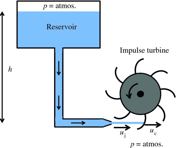
Figure 7.3 Principle of operation of a Pelton impulse turbine. The turbine has a series of cups attached to a revolving wheel. The jet of water impinges on the cups and is deflected so that the water suffers a change in momentum. This produces a tangential force on the wheel that causes it to rotate.
Figure 7.3 shows the water jet of density ρ and volume flow rate Q hitting the cup in the laboratory frame, i.e. in the frame of the (stationary) hydroelectric plant. The cup moves to the right with tangential velocity uc, while the constant velocity of the jet is uj. In the cup's frame of reference, the cup sees the water jet coming towards it with velocity (uj − uc). The shape of the cup is designed so that the water jet is deflected through almost 180°. Hence in the cup's frame of reference we can say that the water suffers a total change in momentum of 2(uj − uc). The change in momentum per unit time and hence the force F experienced by the cup is
Hence the power transferred to the cup is

By differentiating this equation with respect to uc, for constant uj, we see that there is maximum power, Pmax, when

Then substituting for uc in Equation (7.8) we obtain for the maximum power:
This is the same result we would obtain if we were to direct the water jet at a fixed wall and its velocity reduced to zero at the wall (see Equation 6.16). Thus, in this ideal case we have extracted all the power of the water jet and the turbine is 100% efficient. The potential efficiency of impulse turbines can be so high because the water is deflected away from the cups. This is in contrast to a wind turbine where the wind has to flow through the rotor and so its velocity cannot reduce to zero. In practice, large commercial impulse turbines have high efficiencies of ∼90%.
The pressures at the top of the reservoir and at the water jet are the same and equal to atmospheric pressure. And the water velocity at the top of the reservoir can be assumed to be zero as the reservoir has a large surface area. Hence from Bernoulli's equation,

we readily obtain

where h is the difference in vertical height between the top of the reservoir and the water jet, i.e. the head of water. This result assumes that the water has no viscosity. To take viscosity into account, we replace the head of water h by the available head, ha = h − hf (Equation 7.6), to obtain

If the nozzle has area aj, the flow rate Q through the nozzle is equal to ajuj. Then, substituting for Q and the jet velocity uj from Equation (7.11) into Equation (7.9), we see that the maximum obtainable power is given by
The 3/2 exponent of ha emphasises the need to maximise the available head of water.
One way to increase output power is to increase the number of jets striking the turbine cups, as illustrated by Figure 7.4. For n jets, the maximum power is
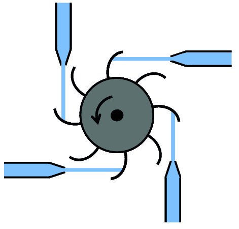
Figure 7.4 The power delivered to an impulse turbine can be increased by the use of additional water jets. Of course, the total flow of water from the jets must be less than the flow of water out of the water reservoir.
Of course, the total flow, Q, of water through the turbine must be less than the net flow of water out of the reservoir.
The overall efficiency of a hydroelectric plant arises from the combination of the turbine efficiency, the efficiency of the electrical generator and the head loss in the penstock. The efficiencies of the turbine and generator are both typically about 90%, while the available head may be 90% of the actual head. Multiplying these factors together, we obtain an overall efficiency of 73%, which is a typical value for a large hydroelectric plant.
7.2 Wave power
Anybody swimming in the sea feels the power of the waves, especially if they are drawn too far away from the coastline. Indeed, ocean waves have the potential to deliver huge amounts of energy; estimates suggest that they could provide a third of the world's energy needs. And they have significant advantages as an energy source. They provide a renewable source of energy, they occur throughout the world's oceans, and waves are, to a degree, more predictable than some other renewable energy sources. Consequently, there have been many schemes to harvest the power of water waves and a number of these schemes have been tried. However, wave power has yet to contribute a significant amount of energy to world demand. The main reason is that an ocean can be a hostile environment. Extraordinarily large waves can occur on occasions and any equipment must be able to withstand the pounding of such waves. Moreover, salt water is corrosive to the mechanical components of the equipment.
Water waves are a familiar phenomenon and have properties that are common to all waves. Indeed, when we visualise a wave we probably think of an ocean wave or a wave breaking on a beach because of their visibility and relatively low speed. Despite their familiarity, however, water waves are quite complicated, more complicated than say a wave on a plucked guitar string. Nevertheless, we can get an understanding of water waves from some basic physics and using reasonable assumptions and simplifications. And we can obtain a good estimate of the power that is delivered by an ocean wave. We begin by describing the general characteristics of wave motion, using transverse travelling waves as an example, as these are the easier to understand. We then extend our discussion to ocean waves.
7.2.1 Wave motion
When we observe a wave it is clear that something, which we may call a disturbance, travels or propagates from one region of a medium to another. This disturbance travels at a definite velocity that is usually determined by the properties of the medium. However, the medium does not travel with the wave. For example, if we tap one end of a solid metal rod, a sound wave propagates along the rod but the rod itself does not move. Rather, the particles of the rod move about their equilibrium positions to which they are bound. Similarly, when we throw a stone into the middle of a pond, the water that is disturbed by the stone does not travel to the edge of the pond and pile up there. Instead, waves propagate because adjacent particles in the medium interact with each other and pass on their energy to their neighbour which, in turn, passes the energy on to its neighbour. We may think of a Mexican wave travelling around a stadium. A spectator jumps up and down as they see their neighbour on one side do the same and this action is propagated around the stadium, but, of course, the spectators do not move away from their seats.
Waves may be either standing waves or travelling waves. The wave on a plucked guitar string is an example of a standing wave. On the other hand, solar radiation consists of electromagnetic travelling waves. As ocean waves are also travelling waves, we will focus our attention on this type of wave. (We will see an example of standing waves in water in our discussion of tidal motion in Section 7.3.2.) Waves are also characterised as being transverse or longitudinal. The wave on a guitar string is a transverse wave, where the displacement of the string is perpendicular to the wave's direction of propagation. By contrast, a sound wave is a longitudinal wave, where the disturbance travels as successive compressions and rarefactions of the air. One of the complications of water waves is that they are a combination of both transverse and longitudinal motions; particles in a water wave trace out ellipses about their equilibrium positions, as we shall see. However, both transverse and longitudinal waves are solutions of the wave equation, which is one of the fundamental equations in physics.
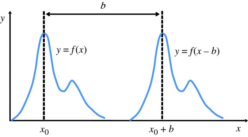
Figure 7.5 Plots of the functions y = f(x) and y = f(x − b). The shapes of the two functions are the same, but y = f(x − b) is displaced by distance b along the positive x-axis with respect to y = f(x).
Imagine that we have a function y = f(x), such as that shown in Figure 7.5. The function has a maximum at x = x0. If we change the variable x to, say, (x − b), we obtain the function y = f(x − b), which is also plotted in Figure 7.5. We see that the shape of this function is the same as before. We have simply displaced this shape a distance b to the right, so that now its maximum occurs at x = (x0 + b). Suppose that we now change the variable x to (x − vt) where t is time and v is a constant:
The value of vt increases linearly with time. Consequently, Equation (7.14) describes a waveform that moves in the positive x direction at a constant rate. Clearly, the product vt must have the dimensions of length and therefore v has the dimensions of length divided by time, i.e. v is a velocity. This is illustrated in Figure 7.6, which shows the waveform described by function y = f(x − vt) at three successive instants of time, separated by time interval δt. The rate at which it moves is its velocity v.
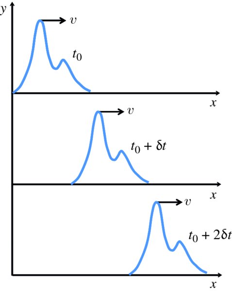
Figure 7.6 The function y = f(x − vt) at three successive instants of time, separated by time interval δt. The rate at which the function moves to the right is the velocity v.
We can generalise the above by saying that when a wave is travelling in the positive x direction, the dependence of the shape of the wave on x and t must be of the general form f(x − vt), where f is some function of (x − vt). We can obtain the shape of the wave by taking a snapshot of it at a particular instant of time; for example at t = 0 when y = f(x). It follows that a wave travelling in the negative x direction must be of the form y = g(x + vt), where g is some function of (x + vt). In general, then, a transverse wave has the form

The one-dimensional wave equation
Equation (7.15) is the general solution of the one-dimensional wave equation. To see this, we start with the function f(x − vt) and change variables to u = (x − vt) to obtain the function f(u), which is a function of u only. Then
and
As ∂u/∂x = 1 and ∂2u/∂x2 = 0, we have
Similarly,
Combining Equations (7.16) and (7.17) we obtain
Similarly, we can readily show that g(x + vt) satisfies the equation
It does not matter that the sign of the velocity has changed between f(x − vt) and g(x + vt) since only the square of the velocity occurs in Equations (7.17) and (7.19). Thus
and hence we can write
This is a fundamental result. Equation (7.20) is the one-dimensional wave equation with the general solution

The wave equation (7.20) and its general solution (7.21) apply to all waves that travel in one dimension. For example, they describe sound waves in a long tube, voltage waves on a transmission line and temperature fluctuations along a metal rod. Consequently, we write the wave equation more generally as
and its general solution as

where ψ(x, t) represents the relevant physical quantity.
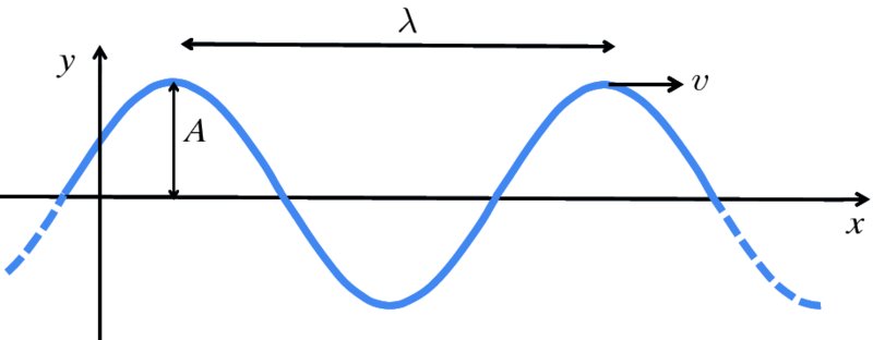
Figure 7.7 The figure illustrates the travelling sinusoidal wave y = Asin 2π[(x − vt)/λ], where λ and A are the wavelength and amplitude of the wave, respectively. The wave propagates along the x-axis and the displacement is along the y-axis, at right angles to the propagation direction. The wave travels at velocity v in the positive x-direction. The dotted parts of the curves indicate that the wave extends to large distance in both directions.
Sinusoidal travelling waves
Sinusoidal waves are important because they occur in many applications of physics and engineering and, indeed, they are used to model ocean waves. In addition, they are important because more complicated wave shapes can usually be decomposed into a combination of sinusoidal waves as described by Fourier analysis. So if we understand sinusoidal waves, we can understand these more complicated waves.
A travelling sinusoidal wave is illustrated in Figure 7.7. The dotted parts of the curves indicate that the wave extends a large distance in both directions. A sinusoidal wave is a repeating pattern. The length of one complete pattern is the distance between two successive maxima (crests), or between any two corresponding points. This repeat distance is the wavelength λ of the wave. The sinusoidal wave propagates along the x-axis and the displacement is along the y-axis, at right angles to the propagation direction. We represent this travelling sinusoidal wave by
where A is the amplitude of the wave. The wave travels at velocity v in the positive x direction. The number of times per unit time that a wave crest passes a fixed point is the frequency, ν, of the wave. ν is equal to the wave velocity v divided by the wavelength λ. Hence we obtain

We see that the important parameters of the wave, wavelength, frequency and velocity are related by this simple equation. The time T that a wave crest takes to travel a distance λ is equal to λ/v, i.e. the reciprocal of the frequency. Hence,

where T is the period of the wave.
It is sometimes convenient to use alternative formulations for a travelling sinusoidal wave. Thus,
where k = 2π/λ and ω = 2π/λv = 2πν, and hence

ω is called the angular frequency of the wave and k is called the wavenumber.
If we consider the displacement of the wave at any particular point, say at x = 0 for the sake of simplicity, Equation (7.27) reduces to y = Asin ( − ωt). We recall that sin ( − θ) = −sin θ. Hence, y = −Asin ωt, which represents simple harmonic motion with angular frequency ω. Hence that point,
and indeed all points along the wave, undergo simple harmonic motion about their equilibrium
positions at frequency ω. Each point on the wave completes one period of oscillation
in time period
 .
.
We have used sine functions to represent waves, but we can equally well use cosine functions such as

since the cosine function is simply the sine function with a phase difference of π/2.
Transport of energy by a wave
Waves transport energy. This is apparent in sound waves that excite our ear drums and in the heat from sunlight. In mechanical waves, such as sound waves and ocean waves, the energy resides in the kinetic energy and potential energies of the particles in the medium. The particles have kinetic energy due to their oscillating motion. They have potential energy because there is a restoring force that pulls them back to their equilibrium positions when they are displaced. As a wave propagates, it carries these energies along with it.
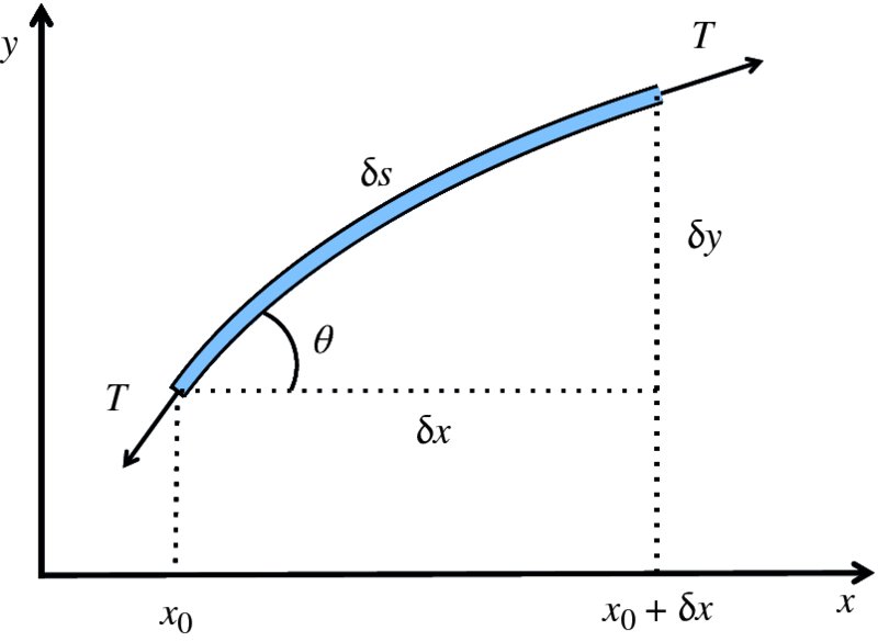
Figure 7.8 Segment of a taut string between x0 and x0 + δx that carries a wave. The directions of the tension T acting on each end of the segment are indicated.
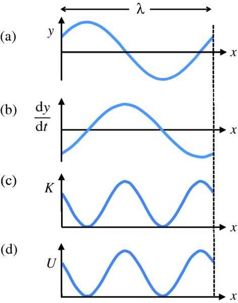
Figure 7.9 (a) Snapshot of a portion of a taut string carrying a travelling sinusoidal wave, over one complete wavelength λ. (b) Variation of the instantaneous velocity dy/dt of the wave. (c) Variation of the instantaneous kinetic energy, K. (d) Variation of the instantaneous potential energy, U.

Figure 7.10 Part of a sinusoidal wave travelling on a taut string at velocity v towards the right. (a) Displacement of the wave. (b) Energy distribution in the wave. The energy is transported with the wave at velocity v.
Dispersion of waves, phase and group velocities and wave groups
In some media, the velocity v of a transmitted wave does not depend on its wavelength, i.e.
 , where the symbols have their usual meanings. Sound waves in air are an example of
this. Such media are said to be non-dispersive. In some other media, the velocity of a wave does depend on wavelength. Perhaps the
most familiar example of this is light waves in glass. Because different wavelengths
travel at different velocities in glass, white light is dispersed by a glass prism
into the colours of the rainbow. Such media are said to be dispersive. In the case of ocean waves, it is found that the velocity of waves on shallow water
is independent of wavelength. However, for waves on deep water, the velocity does
depend on wavelength.
, where the symbols have their usual meanings. Sound waves in air are an example of
this. Such media are said to be non-dispersive. In some other media, the velocity of a wave does depend on wavelength. Perhaps the
most familiar example of this is light waves in glass. Because different wavelengths
travel at different velocities in glass, white light is dispersed by a glass prism
into the colours of the rainbow. Such media are said to be dispersive. In the case of ocean waves, it is found that the velocity of waves on shallow water
is independent of wavelength. However, for waves on deep water, the velocity does
depend on wavelength.
In our discussion of sinusoidal waves so far, we considered the case of a monochromatic wave, i.e. one with a single, well defined wavelength and frequency. In most practical
situations, however, we usually deal with a group of waves that have different wavelengths. In a storm, for example, waves of different
wavelength are generated. On deep water these waves travel at different velocities;
at some distance from the storm it is found that water waves of long wavelength reach
an observer before waves of shorter wavelength do. And experienced sailors can use
this to deduce how far the storm is away. When we deal with a group of waves containing
different wavelengths, two different velocities arise. These are the phase velocity vp and the group velocity vg as we will shortly describe. The distinction between the two velocities is important
because when we have a group of waves, the energy is carried at the group velocity. In our previous discussion of sinusoidal waves,
 , there was a single wavelength λ. In that case, v is the phase velocity and the concept of group velocity did not arise.
We illustrate the difference between phase and group velocities by considering the superposition of two sinusoidal waves, ψ1 and of ψ2, having slightly different frequencies that travel in a dispersive medium. The frequencies of the waves are ω1 and ω2, respectively, with corresponding wavenumbers k1 and k2:

where A is the amplitude of both waves. When we sum these two waves together we obtain
As the medium in which the two waves travel is dispersive, they travel at different velocities given by v1 = ω1/k1, and v2 = ω2/k2, respectively. We let
where k0 and ω0 are the mean values of the wavenumbers and frequencies, respectively. As the differences between ω1 and ω2 and between k1 and k2 are small, we write
We can then write Equation (7.40) as

where

Equation (7.43) represents a wave
 that has frequency ω0, wavenumber k0 and velocity vp given by

where vp is the phase velocity. This wave looks like a sinusoidal wave but one whose amplitude A(x, t) is modulated according to Equation (7.44). This modulation forms an envelope that contains the sinusoidal-like wave.
Propagation of the modulated wave is illustrated in Figure 7.11. This shows plots of
 at successive instants of time that are separated by time interval δt. The wave is shown as a solid line, while the envelope of the wave is represented
by the dashed lines. As can be seen, the envelope travels forward with the wave but
it does so at a different velocity. This can be discerned from the relative movement
of a particular maximum of the wave, marked by the vertical arrows, with respect to
a particular maximum of the envelope, which is marked by the black dot. While the
crest of the wave travels at the phase velocity vp = ω0/k0, the envelope travels at the group velocity vg.
at successive instants of time that are separated by time interval δt. The wave is shown as a solid line, while the envelope of the wave is represented
by the dashed lines. As can be seen, the envelope travels forward with the wave but
it does so at a different velocity. This can be discerned from the relative movement
of a particular maximum of the wave, marked by the vertical arrows, with respect to
a particular maximum of the envelope, which is marked by the black dot. While the
crest of the wave travels at the phase velocity vp = ω0/k0, the envelope travels at the group velocity vg.
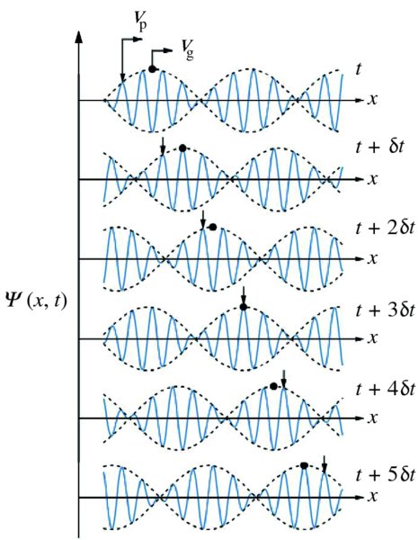
Figure 7.11 The propagation of the modulated wave
 in a dispersive medium. The wave is shown at several successive instants of time,
separated by time interval δt. The wave is shown as the solid line and is contained within the envelope of the
modulation, which is represented by the dashed black lines. The vertical arrows indicate
a particular crest of the wave, which travels at the phase velocity vp. The black dots indicate a particular maximum of the envelope, which travels at group
velocity vg. In this example, vp > vg and so the wave crest moves forward through the envelope as the wave propagates.
This can be seen from the changing relative positions of the arrows and the bold dots.
in a dispersive medium. The wave is shown at several successive instants of time,
separated by time interval δt. The wave is shown as the solid line and is contained within the envelope of the
modulation, which is represented by the dashed black lines. The vertical arrows indicate
a particular crest of the wave, which travels at the phase velocity vp. The black dots indicate a particular maximum of the envelope, which travels at group
velocity vg. In this example, vp > vg and so the wave crest moves forward through the envelope as the wave propagates.
This can be seen from the changing relative positions of the arrows and the bold dots.
We can obtain an expression for the group velocity in the following way. Consider for a moment the maximum in the envelope marked with the black dot in the top waveform shown in Figure 7.11, at time t. At this point in the envelope, the function A(x, t) must have its maximum value and this occurs when the cosine term cos [xΔk − tΔω] = 1, with [xΔk − tΔω] = 0. Indeed, as the envelope moves along with the wave, it will always be the case that xΔk − tΔω = 0 at the maximum in the envelope; the values of x and t change but they always obey this equation. By differentiating this equation with respect to t and remembering that Δk and Δω have fixed values, we obtain the group velocity vg at which the maximum in the envelope, and indeed the whole envelope, travels.
Hence,
As ω is a function of wavenumber k in a dispersive medium, we write Equation (7.46) as
Using Taylor's theorem, we have
where
 (Equation 7.42). When Δk is small compared with k0, we need only retain linear terms in Equation (7.48), which we can write as
Substituting for k0 and Δk from Equations (7.41) and (7.42), respectively, we obtain
and hence Equation (7.47) for the group velocity becomes
We see that the group velocity is equal to the derivative of ω with respect to k, evaluated at the wavenumber k0.
We have obtained expressions for the phase and group velocities using the example of the sum or superposition of just two single-frequency sinusoidal waves. These expressions, however, apply to any group of waves so long as their frequency range is narrow compared with their mean frequency. Thus, for the general case, we define the phase velocity, vp as

and the group velocity, vg, as

Wave groups
We can imagine summing a large number of sinusoidal waves that cover a narrow range of angular frequencies centred about a mean frequency ω0. In that case we would obtain a wave group or wave packet, which looks like that shown in Figure 7.12. Over a particular, narrow spatial range, all the individual sinusoidal waves are in phase and interfere constructively. Outside this narrow range, however, the waves rapidly go out of phase and interfere destructively, reducing the wave amplitude to zero. As the individual sinusoidal waves travel along the propagation direction, they do so at slightly different velocities in a dispersive medium. The result is that the narrow spatial region over which they interfere travels at a different velocity to the individual waves. Again we can think of the resultant waveform as a sinusoidal-like wave of frequency ω0 and corresponding wavenumber k0 whose amplitude is heavily modulated. As before, the wave travels at the phase velocity vp = ω0/k0, and the envelope containing the wave travels at the group velocity vg = dω/dk.
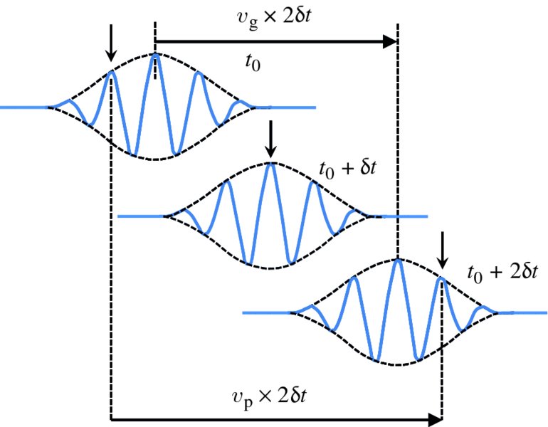
Figure 7.12 The figure shows a wave group that results from summing together a large number of sinusoidal waves that cover a narrow range of frequencies centred about a mean frequency. The figure shows the wave group at three successive instants of time, separated by time interval δt for the case where the phase velocity vp is larger than the group velocity vg. A crest of the wave, indicated by the arrows, travels a distance 2vp × δt, while the envelope travels a distance 2vg × δt. We can imagine crests of the wave appearing at the back (left-hand) side of the envelope, passing through the envelope and disappearing at the front of the envelope. As the amplitude is only non-zero within the spatial extent of the group, it follows that the wave energy is transported at the group velocity vg.
Figure 7.12 shows the wave group at three instants of time, separated by time interval δt, for the case where the phase velocity vp is larger than the group velocity vg. A crest of the wave, indicated by the arrows, travels a distance vp × 2δt, while the envelope travels a distance vg × 2δt; the wave crest moves through the envelope. We have seen that the energy contained in a wave is proportional to the square of its amplitude (see Equation 7.38). Looking at the wave group in Figure 7.12 we see that the amplitude is only non-zero within the spatial extent of the group as defined by its envelope. It follows that the energy is transported at the same velocity as for the envelope of the wave, i.e. at the group velocity.
7.2.2 Water waves
Physical characteristics of water waves
Water waves are generated by wind passing over the surface of the sea. On a calm sea, the wind has little grip on the water. As it moves over the water surface, however, the wind starts to form eddies and small ripples. Once the surface becomes uneven in this way, the wind has an increasing grip on it. It becomes easier for the wind to transfer its energy to the water and the ripples turn into small waves. As long as the wind velocity is greater than the velocity of the waves, there is a transfer of energy from the wind to the waves and the height of the waves steadily increases. There is, however, a limit to this energy transfer and when a wave has absorbed the maximum possible energy from the wind, it is said to be fully developed. The eventual height of a wave is determined by wind velocity, the duration of time the wind has been blowing, and the area of contact between the wind and the water, which is called the fetch. The depth and topography of the seafloor, which can focus or disperse the energy of the waves, also affect the wave height. And the greater the wave height, the greater is the energy that is contained in the wave.
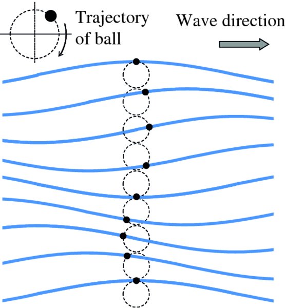
Figure 7.13 The figure illustrates the motion of a small ball floating on a water surface at nine equally spaced instants of time as a wave passes by. As the wave moves forward, so too does the ball. However, as the ball reaches the wave trough, it starts to move backwards and eventually ends up at its initial position, which coincides with the position of the following wave crest. The ball moves in a uniform circular motion in a clockwise direction as shown in the inset of the figure and there is no net forward movement of the ball as the wave propagates. Notice that the ball never leaves the surface of the water, which is depicted as the blue lines.
One important characteristic of water waves that we have already noted is that they
exhibit both transverse and longitudinal motion. Imagine that we watch a small ball
that floats on the surface of deep water. What we see as a wave passes by is that
the ball bobs up and down on the water. What we also see is that the ball moves forwards
and backwards along the propagation direction of the wave. This is illustrated by
Figure 7.13, which shows the position of the ball at nine equally spaced instants of time. The
ball never leaves the surface of the water, which is shown in blue. Initially it is
on the crest of the wave. As the wave moves forward, the ball does too. However, as
the ball reaches the wave trough, it starts to move backwards and eventually ends
up at its initial position, which coincides with the position of the following wave
crest. The ball moves in a uniform circular motion in a clockwise direction, and there
is no net forward movement of the ball as the wave propagates. This orbital motion
of the ball is in contrast to the situation for waves on a taut string, where the
motion of each particle of the string is confined to the transverse direction. The period of the orbital motion of the ball,
 , is equal to the period of the wave,
 , and hence the angular frequency, ω, of the circular motion is given by

where v is the wave velocity and λ is the wavelength. Ocean waves typically have wavelengths within the range of tens to hundreds of metres and periods of typically 5–20 s.
We have a similar situation for the water particles on the surface of deep water when a wave passes by. This is illustrated in Figure 7.14, which shows the motion of a number of water particles that are located on the water surface; the surface is shown in blue. The figure shows the positions of these particles at three equally spaced instants of time. We see that as a wave passes by, the water particles on the surface move clockwise in circular orbits. Again there is no net movement of the water particles in the forward direction. There is a phase difference between the respective motions of the water particles and as a water particle falls when a wave crest passes it by, so the next particle rises to take its place on the crest.
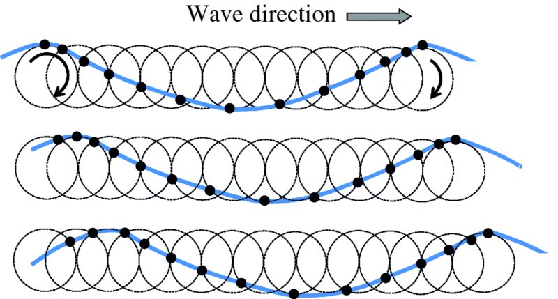
Figure 7.14 Motion of a number of water particles that are located on the water surface, which is shown in blue. The figure shows the particles at three equally spaced instants of time. All the particles move clockwise in circular orbits, but there is a phase difference between their respective motions. As a water particle falls when a wave crest passes it by, so the next particle rises to take its place on the crest.
The circulating motion of the water particles results in a wave profile that is called a trochoid. A trochoid is a curve that can be generated as illustrated in Figure 7.15. This shows a circle of radius R that rolls anti-clockwise along the heavy horizontal line, keeping in contact with the line. The point A that is at a distance H from the centre of the circle traces out a trochoid as shown by the blue curve. The distance between adjacent maxima is equal to 2πR and the amplitude of the curve is equal to H. As can be seen, the shape of the trochoid resembles a sinusoidal wave, and a sinusoidal wave of wavelength 2πR and amplitude H is shown for comparison. Water waves are often modelled as sinusoidal waves, which we will do, because these are easy to handle mathematically.
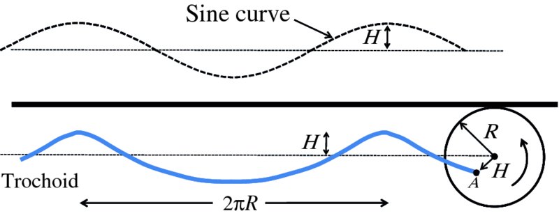
Figure 7.15 The circulating motion of particles in a water wave results in a wave profile that is described as a trochoid. A trochoidal curve can be generated as shown in this figure. Here, the circle of radius R rolls anti-clockwise beneath the black horizontal line. The point A, at a distance H from the centre of the circle, traces out a trochoid as indicated by the blue curve. As can be seen, the shape of the trochoid resembles a sinusoidal wave of wavelength 2πR and amplitude H.
The water particles below the surface of deep water also move in uniform circular motion, as illustrated in Figure 7.16. However, the orbital radius r decreases exponentially with vertical distance z below the surface and is given by

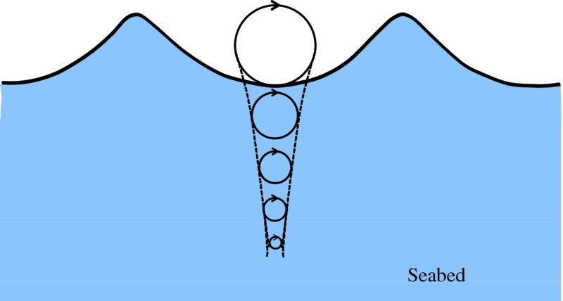
Figure 7.16 In a deep-water wave, the water particles that lie below the water surface also move in a uniform circular motion, but the orbital radius decreases exponentially with vertical distance below the surface.
where H is the amplitude of the circular wave motion at the surface and k is the wavenumber
 . Thus, by the time z ∼λ/2, the radius of the orbit has reduced almost to zero. One aspect of this rapid
decrease in r is that at depths below about λ/2, the water is not appreciably affected by the motion
of the waves. So, a diver below this depth in deep water would not experience any
wave motion. And buoyancy tanks used to support say an offshore oil rig in deep water
(see Figure 7.17) are not appreciably affected by waves if their depth is greater than about half
the wavelength of the waves.
. Thus, by the time z ∼λ/2, the radius of the orbit has reduced almost to zero. One aspect of this rapid
decrease in r is that at depths below about λ/2, the water is not appreciably affected by the motion
of the waves. So, a diver below this depth in deep water would not experience any
wave motion. And buoyancy tanks used to support say an offshore oil rig in deep water
(see Figure 7.17) are not appreciably affected by waves if their depth is greater than about half
the wavelength of the waves.
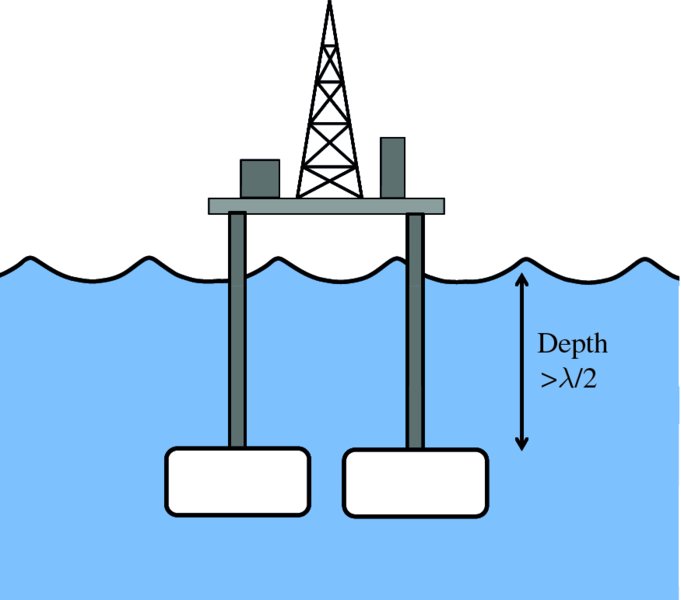
Figure 7.17 As the radius of orbiting water particles in deep water falls of exponentially, the water at depths below about λ/2 is not affected by the motion of the waves. Hence, buoyancy tanks used to support, say, an offshore oil rig in deep water are not appreciably affected by waves if their depth is greater than about half the wavelength of the waves.
For the case where the water is shallow, i.e. where the water depth d < λ/2, the water particles are affected by the presence of the seabed. Then the water particles move in elliptical orbits as shown in Figure 7.18. As the depth of a water particle increases, its vertical component of velocity decreases but its horizontal component remains the same. This explains why the ellipses become flatter towards the seabed. In this case, a diver close to the shore in shallow water, would feel the horizontal motion of the waves.

Figure 7.18 In shallow water, the water particles in a wave are affected by the presence of the sea bed. This results in the particles moving in elliptical orbits. As the depth of a water particle increases, its vertical component of velocity decreases but its horizontal component remains the same, and so the ellipses become flatter towards the sea bed.
Velocity of a water wave
We have seen that the motion of the particles in a water wave is strongly influenced by the water depth d. The velocity of a water wave is also strongly influenced by water depth. We will consider two extremes: shallow-water waves and deep-water waves. Waves on shallow water, i.e. d < λ/2, are the easiest to analyse and we deal with this case first. In our discussions of both types of water waves, we make the following assumptions:
- the water is incompressible;
- the water has no viscosity;
- any variation in the height of the water as the wave passes by is small compared with the depth of the water and small compared with the wavelength of the wave;
- the seabed is level.
Water waves on shallow water, d < λ/2
We describe shallow-water waves in terms of a one-dimensional model in which the waves propagate along the x-axis and the wavefronts are linear, i.e. the wave crests and troughs are linear and perpendicular to the propagation direction. Thus the height, h, of the water varies only along the x-axis. In Figure 7.19 we show the situation where the water is still and the water surface is flat. We imagine the water to be divided into thin slices, each contained between two vertical sides. These slices have width δx along the x-axis, length l along the wavefront, and height h0, equal to the depth of the still water. The width δx of the slices shown in Figure 7.19 is exaggerated for the sake of clarity. In this model, there can be no flow of water into or out of the slices, i.e. the volume of the slices remains constant. When the surface of the water is perturbed by a wave, the slices change shape. In particular, the height, h, of a slice changes to follow the profile of the wave. And as the volume of the slice does not change, the slices will expand and contract as the wave passes by. However, the model assumes that the sides of the slice remain vertical.
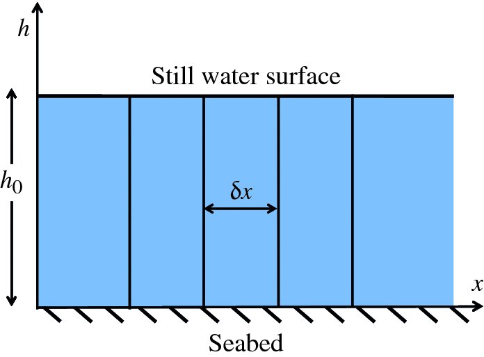
Figure 7.19 In considering wave motion, we imagine shallow water to be composed of thin slices of water, each contained between two vertical sides. These slices have width δx along the x-axis, length l along the wavefront, and height h0, equal to the depth of the still water. The width δx of the slices is exaggerated for the sake of clarity. When the surface of the water is perturbed by a wave, the slices change shape to follow the profile of the wave. However, the volume of each slice remains constant.
Figure 7.20 illustrates the situation where a wave propagates along the water surface. It shows how an unperturbed slice of water is perturbed to follow the wave profile. We are assuming that any variation in the height of the water is small compared with the depth of the water and the wavelength of the wave. Hence, we neglect any variation in the height of the perturbed slice across its width. Then, if the two sides of the slice are displaced by ξ1 and ξ2, respectively, we have

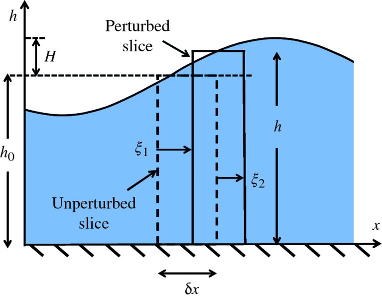
Figure 7.20 The figure illustrates a wave propagating along the surface of shallow water. It shows how a slice of the water is perturbed to follow the wave profile. The height of the slice increases to h and the width changes to δx + (ξ2 − ξ1). Any variation in the height of the water is small compared with the depth of the water and the wavelength of the wave. Hence, we neglect any variation in the height of the perturbed slice across its width.
as the volume of the slice is constant. Differentiating this equation with respect to time t, we obtain
We take the distances ξ1 and ξ2 to be small in comparison to δx and neglect them. Moreover, as we are assuming that any variation in the height of the water is small compared with the depth h0 of the unperturbed water, we can replace h by h0 in the second term of Equation (7.56), which then becomes
The derivatives
 and
and
 are just the velocities of the two sides of the slice, vx1 and vx2 respectively:
In the limit δx → 0, we obtain
We thus have a relationship between the temporal derivative of the height h of the slice and the spatial derivative of its horizontal velocity vx.
We can obtain another relationship between these derivatives by considering the difference in hydrostatic pressure resulting from the variation in height of the water surface. Considering Figure 7.21, we see that the difference in pressure p across the slice is given by

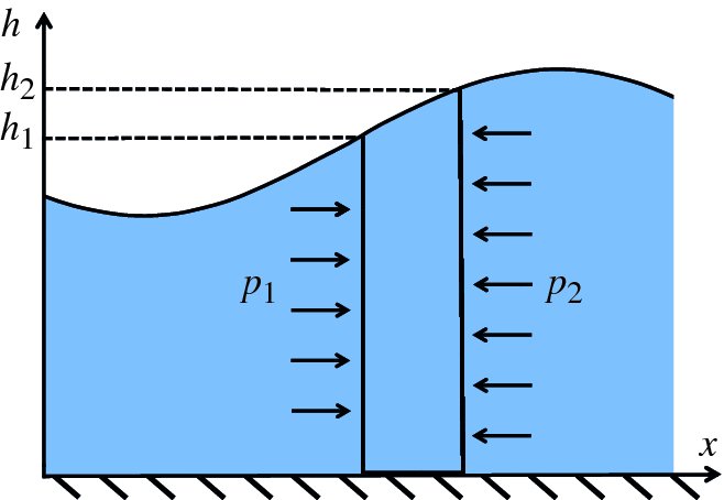
Figure 7.21 This figure illustrates the difference in hydrostatic pressure across a perturbed slice of water resulting from the variation in height of the water surface as a wave passes by.
where ρ is the density of water and g is the acceleration due to gravity. This pressure difference results in a net force on the slice equal to (p1 − p2)h0l, acting in the positive x direction. Taking the volume of the slice to be δxh0l, we have, from Newton's second law:
This simplifies and rearranges to
Then in the limit δx → 0, we obtain

Differentiating this equation with respect to x, gives
and differentiating Equation (7.58) with respect to t, we obtain
Since
we have
This is a statement of the wave Equation (Equation 7.22), with phase velocity vp given by
We see that the phase velocity of shallow-water waves depends upon the depth of the water. For example, if the water depth is 10 m, vp ≈ 10 m/s.
We emphasise that the motion of shallow-water waves occurs predominantly in the horizontal direction and that vertical motion is relatively small by comparison. This is consistent with our picture of water particles following rather flat, elliptical orbits in shallow water (see Figure 7.18).
Water waves on deep water, d > λ/2
Water waves on deep water are more difficult to analyse, but we can use a dimensional argument to deduce an expression for the wave velocity. For this case, we suppose that the phase velocity depends on wavelength λ and on the acceleration due to gravity g, i.e.

Dimensionally, this gives
Equating coefficients for length and time, we readily obtain

In this case, we see that the phase velocity has a strong dependence on wavelength.
Further analysis shows that the constant of proportionality is
 . Hence,
For example, if the wavelength is 250 m, vp ≈ 20 m/s.
Energy of a water wave
In Section 7.2.1 we determined the energy in a wave on a taut string by considering the potential and kinetic energies of a segment of the string as it oscillates about its equilibrium position in simple harmonic motion. For a wave on a taut string, the tension in the string provides the restoring force on the displaced segments. For water waves, it is gravity or surface tension that provides the restoring force, although, as we have already seen, the wavelengths of the ocean waves that we are interested in are too long for them to be appreciably affected by surface tension. Again, we will deal with the two separate cases of waves on shallow water and waves on deep water.
Waves on shallow water
As before, we consider a thin slice of water that, in the absence of a wave, has width δx along the propagation direction, length l along the wavefront, and height h0. As a wave passes by, the slice is perturbed so that its height increases from h0 to h, its width becomes (δx + ξ2 − ξ1) and it has horizontal velocity vx, as illustrated by Figure 7.22. Again, we ignore any variation in wave height across the width of the perturbed slice.
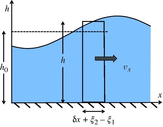
Figure 7.22 A perturbed slice of shallow water gains potential energy because its centre of mass rises from h0/2 to h/2. It also has kinetic energy because it has horizontal velocity vx.
The mass of the unperturbed slice is ρδxlh0 and its centre of mass is at height
 above the seabed. Thus its potential energy with respect to the seabed is
where ρ is the water density. Similarly, the potential energy of the perturbed slice is
Again, the distances ξ1 and ξ2 are small in comparison to δx and we neglect them. The perturbed slice has thus gained an amount of potential energy δU given by
Note that if (h − h0) is a negative quantity, i.e. h < h0, the potential energy must also increase. As the total volume of the water in the ocean is constant, any reduction in the height of the slice must be accompanied by a rise in the water level elsewhere and an equivalent increase in potential energy.
In order to find the total potential energy, Utotal, that is contained within a wavelength of the wave, we integrate over all the slices in a wavelength λ. In the limit δx → 0, this is given by the integral
If we model the water wave as a sinusoidal travelling wave that propagates along the water surface, we have

where H is the wave amplitude. Then
The integral has the value λ/2 and hence the total potential energy in wavelength λ over a length l of the wavefront is given by

and hence the potential energy per unit area of the seabed is
The slice also has kinetic energy δK as it is moving along the x-axis with velocity vx, where
to a good approximation. It is useful to obtain an expression for δK in terms of the height h of the slice so that we can compare its kinetic and potential energies. We have already obtained the following relationship for waves on shallow water:
The function h(x,t) describing the water wave must be of the general form: h(x, t) = h(x − vpt), where vp is the phase velocity. Then:
Substituting for
 from Equation (7.74) into Equation (7.62), we obtain
Integrating this equation with respect to t, we have
For still water, when h = h0, vx = 0. Hence we can write
Substituting for vx from this equation into Equation (7.73), we obtain the following expression for the kinetic energy δK of the slice:
We recall that the phase velocity vp of a shallow-water wave is given by
Hence, substituting for vp in Equation (7.78) we obtain
Comparing Equations (7.115) and (7.101), we see that the potential and kinetic energies of the slice are equal, just as the potential and kinetic energies of a segment of a taut string are equal when a wave propagates. Thus we can immediately say that the kinetic energy per unit area of seabed is

The total energy per unit area of seabed Etotal, i.e. the energy density, is then
We emphasise again that the predominant motion of shallow-water waves is in the horizontal direction and that the kinetic energy resides in this horizontal motion.
Waves on deep water
In the case of waves on deep water, the water particles move in circular motion. And this must be taken into account in determining the kinetic energy of a wave. We can do this in the following way. Figure 7.23 shows an elemental volume of water in the wave that is at a vertical depth z below the still-water surface. The width, length and height of the elemental volume are dx, dl and dz, respectively; dl is measured along the wavefront. Figure 7.23 is a snapshot of the element at the instant of time when its instantaneous velocity v is pointing upwards.
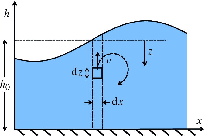
Figure 7.23 The water particles in a wave on deep water follow circular paths with velocity v = rω, where r is the radius and ω is the angular frequency. The figure shows an elemental volume of water in the wave at the instant of time when its instantaneous velocity v is pointing upwards.
The mass of the element is ρdldzdx, where ρ is the water density. Its kinetic energy is given by
as it is moving in a circular motion with velocity v = rω, where r is the radius and ω is the angular frequency. Substituting for r = He− kz, from Equation (7.54), we obtain
To obtain the total kinetic K energy in a vertical slice of water of width dx we integrate this equation from z = 0 to z = ∞. (We can use the limit z = ∞ because we are dealing with deep-water waves where z is large and where the term e− 2kz decreases very rapidly with z. Then

To find the total kinetic energy in a wavelength λ of the wave along a length l of the wavefront, we integrate this equation over dx from x = 0 to λ, and over dl from l = 0 to l:

The result is
We have
 and ω = 2πvp/λ (see Equation 7.28). The phase velocity of waves on deep water is given by
 (Equation 7.68). Thus we obtain
 and, substituting for k and ω2 in Equation (7.86), we have
and the kinetic energy per unit area of the seabed is

This is the same result that we obtained for the kinetic energy density of a shallow-water wave.
The potential energy per unit area of seabed for a deep-water wave is obtained in exactly the same way as that for a wave on shallow water with the same result:
Thus the total energy Etotal per unit area, i.e. the energy density in a deep-water wave is equal to
 , just as it is for shallow-water waves.
Power of a water wave
From Equation (7.81) the wave energy per unit wavefront, i.e. per metre, is

This result applies to both shallow- and deep-water waves. The time it takes for one wavelength of the wave to pass a given point is equal to the wavelength divided by the velocity of the wave. When we are dealing with a group of waves, as we usually are in ocean waves, the wave energy is transported at the group velocity vg (see Section 7.2.1). Hence, the rate at which energy per unit wavefront passes a given point, i.e. the wave power P per unit wavefront is
For waves on shallow water, the phase velocity
 (Equation 7.66). Then,
and we see that the group velocity is equal to the phase velocity for shallow-water waves. Hence the wave power per unit length of wavefront is given by
Water waves on deep water, on the other hand, are dispersive with phase velocity
 (Equation 7.68), which gives

Hence,
and in this case, the group velocity is equal to half the phase velocity. Hence the power P delivered by a deep water wave is given by
We have used sinusoidal waves of amplitude H to model water waves. In this case the wave height, trough to crest, is equal to twice the amplitude, i.e. equal to 2H. In reality, there is a distribution of wave heights. In oceanography this is taken into account by using a representative height Hs, which is called the significant wave height. It is defined as the mean height of the highest third of the waves and is a parameter that can be measured empirically. In terms of this parameter, the expression for the wave power per unit length of wavefront for deep-water waves is
7.2.3 Wave energy converters
A machine that harnesses wave energy is known as a wave energy converter. A large number of different methods of wave energy conversion has been proposed and some typical methods are described below. No main design has been adopted, unlike the situation for wind power where most wind turbines have adopted the same basic design. Indeed, wave power technology is a few decades behind wind power technology. However, because of the issue of climate change, there is growing interest in wave power, which has significant advantages: it is a renewable energy source, it has the potential to deliver huge amounts of energy, and it does not produce any pollutant or greenhouse gases in operation. However, until one or two main designs are established, it seems unlikely that large-scale manufacture of wave energy convertors will begin, and at present there are no commercial-scale wave energy conversion systems in operation around the world.
The challenges for wave energy converters arise from the fact that they are usually located out to sea. There they must be able to withstand storm conditions with energies hundreds of times larger than they were designed to capture, while seawater is corrosive to mechanical components. Furthermore, the electrical power generated by the converter must be transported to land, as is also the case for offshore wind turbines. In addition, waves at a particular location vary in height, velocity and direction and so it is a challenge to find an optimum design for all sea conditions. It may be that two main designs will emerge, one for deep water and one for shallow water found closer to shore.
Wave power can be expected to be greatest in those regions where strong winds blow consistently in a particular direction. We saw in Section 6.2 that increased wind activity is found between latitudes of 30° and 60° and so the best sites for wave power are found in these regions. Important research centres for wave power are also located in these regions, and Scotland and Oregon on the north west coast of North America have important such centres.
Overtopping devices
An overtopping device is perhaps the simplest wave energy conversion system conceptually. The principle of operation is illustrated in Figure 7.24. Waves break over a sea wall, whose height is above the mean sea level, and the water is collected in a reservoir. The collected water is returned to the sea via a turbine, which drives an electrical generator in a similar way to a conventional hydroelectric plant. In order to maximise the amount of collected water, a tapered channel funnels the incoming waves into the reservoir. Friction between the waves and the sides of the channel is small and so there is insignificant dissipation of wave energy. As the width of the channel decreases, the height of the waves increases and this enables more of the waves to reach above the sea wall. Such a system, called the tapered channel (Tapchan) method was successfully demonstrated in Norway in 1985, and delivered a nominal electrical power of 350 kW. As there are few moving parts, maintenance costs are relatively low and in addition, the reservoir provides in-built energy storage. The main disadvantage of this system is the large capital building cost.
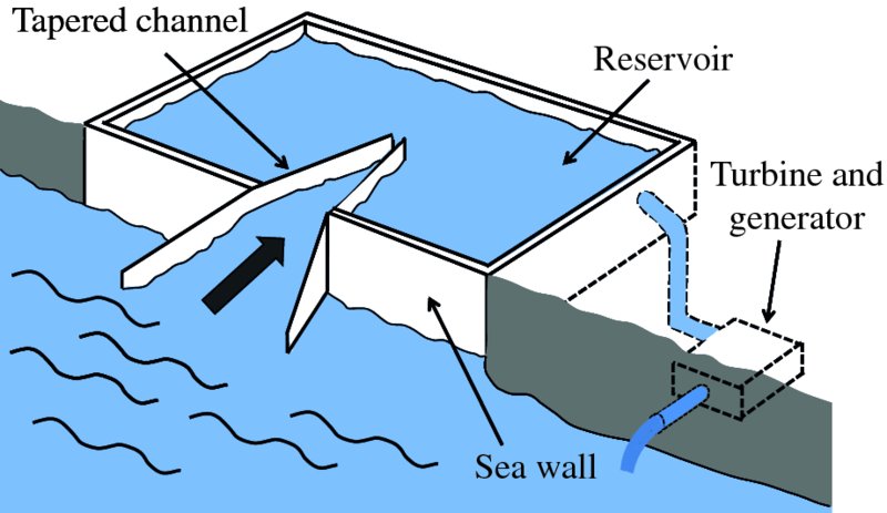
Figure 7.24 In an overtopping energy converter, waves break over the sea wall whose height is above the mean sea level and the water is collected in a reservoir. The collected water is returned to the sea via a turbine, which drives an electrical generator. In order to maximise the amount of collected water, a tapered channel funnels the incoming waves into the reservoir.
Oscillating water column systems
The principle of this system is illustrated in Figure 7.25 for the case of a shore-based application; analogous systems can be located offshore. The system has an enclosed air chamber that is securely mounted on the land side. The chamber has an open bottom that is submerged in the sea, while the other end is connected to a turbine. The water level in the chamber rises and falls in synchronism with the incoming waves and sets up an oscillating column of air. As a result, the air in the chamber is forced forwards and backwards through the turbine and this causes the turbine to rotate. The turbine is a Wells turbine, which has the important feature that it is driven in the same direction by both forward and backward air flow. The turbine is connected to a conventional generator that produces the electricity.
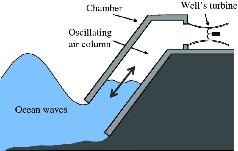
Figure 7.25 Operating principle of an oscillating water column energy converter. The water level in the chamber rises and falls in synchronism with the incoming waves and sets up an oscillating column of air. As a result, the air in the chamber is forced forwards and backwards through a Well's turbine and this causes the turbine to rotate. The turbine is connected to a conventional generator that produces the electricity.
The channel that connects the air chamber to the turbine has a reducing cross-sectional area. This increases the air speed and gives better matching of the relatively slow motion of the water to the fast rotation of the turbine without mechanical gearing. The shape and size of the air chamber determine its frequency response to the incoming waves, i.e. resonance frequency. These parameters can be tuned to best match the frequency of the waves so that maximum power is extracted from the waves. Important advantages of such an onshore device are that the turbine is remote from the corrosive action of the seawater and there is no need for underwater electrical components or cables. An example of this type of energy converter is Limpet, which is installed on the Scottish Isle of Islay. It was the first commercial wave energy converter to be connected to the UK national grid and it has provided much of Islay's electricity needs since it became operational in the year 2000.
The Edinburgh Duck
The Edinburgh Duck, also known as Salter's Duck, was one of the earliest wave energy converter designs, following the oil crisis of the 1970s. The device is shown schematically in Figure 7.26. It floats in the water and as waves pass beneath it, the duck rocks back and forth – hence its name. This rocking motion absorbs the mechanical energy in the wave. The shape of the duck is critical to maximise the amount of energy absorbed and was designed by Stephen Salter at Edinburgh University. Theoretically this design has an energy conversion efficiency of 90%, although inevitably in real sea conditions the efficiency would be lower than this. The absorbed energy is converted into electrical energy by a combination of hydraulic rams and an electrical generator that are contained within the duck.
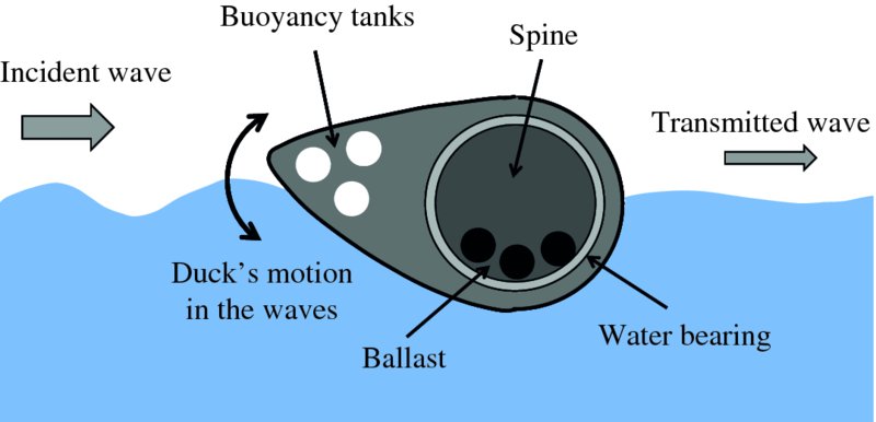
Figure 7.26 The Edinburgh duck, also known as Salter's Duck. It floats in the water and as waves pass beneath it, the duck rocks back and forth. This rocking motion absorbs the mechanical energy in the wave. The absorbed energy is converted into electrical energy by a combination of hydraulic rams and an electrical generator that are contained within the duck.
The original duck never went into commercial operation, partly because of the fall in oil prices in the 1980s. However, development of the original duck and duck-like devices has continued, spurred on by the increasing interest in renewable energy sources. It is envisaged that a long string of, say, 24 duck-like devices could be linked together through a central spine and moored parallel to the incoming wavefronts. Clearly, a wave energy converter captures energy from the waves. As a result the waves will be of lower height in the region behind the wave power device, and this may have environmental effects.
Pelamis energy converter
Perhaps the most developed wave energy converter is the Pelamis system. It is a semi-submerged, articulated structure as illustrated schematically in Figure 7.27. This snake-like structure is 150 m long and consists of long cylindrical sections that are linked to shorter sections by hinged joints. The short sections contain the machinery that generates the electricity. Pelamis is tethered to the seabed by an anchor chain and undulates up and down with the motion of the waves, conforming to the local shape of the wave. It is partially free to rotate and can align itself with the direction of the waves for maximum absorption of energy.
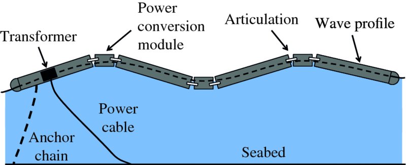
Figure 7.27 Illustration of the Pelamis energy converter, which is a semi-submerged, articulated structure. It consists of long cylindrical sections that are linked to shorter sections by hinged joints. The short sections contain the machinery that generates the electricity. Pelamis is tethered to the seabed by an anchor chain and undulates up and down with the motion of the waves, conforming to the local shape of the wave. The undulating motion of the device is converted into electrical energy by a combination of hydraulic rams and an electrical generator.
As the Pelamis undulates with the waves, hydraulic pumps in the power-conversion sections drive high-pressure fluid through hydraulic motors, as illustrated in Figure 7.28; the action of an individual motor is illustrated schematically in Figure 7.29. The high-pressure fluid passes through the input port and travels between the gear teeth and the motor housing, before leaving via the output port. This flow of fluid causes the gears to rotate. The shaft of one of the gears is connected to an electrical generator and its output is connected to a transformer that delivers three-phase electricity at a voltage of 15 kV. This is fed down an electrical cable to the seabed and another high voltage cable transfers the electricity to shore. For a wave height of 5 m, the Pelamis can produce ∼750 kW of electricity. A Pelamis has been successfully tested at the European Marine Energy Centre in Orkney, Scotland, and another has been installed off the coast of Portugal. A photograph of a Pelamis wave energy converter at sea is shown in Figure 7.30.
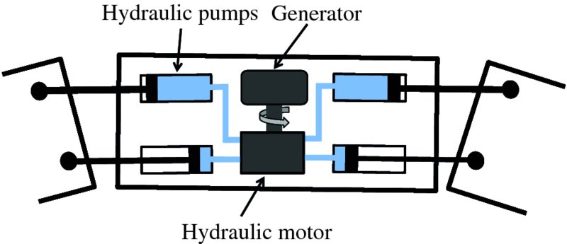
Figure 7.28 Schematic diagram of a hydraulic motor. As the sections of the Pelamis undulate with the action of the waves, high-pressure fluid is forced through pumps that are connected to a hydraulic motor. These hydraulic components are located in the short sections of the Pelamis.
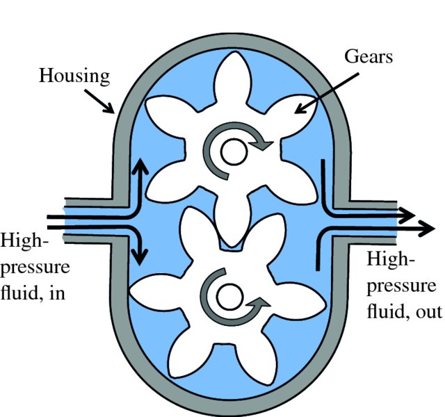
Figure 7.29 Action of a hydraulic motor. High-pressure fluid passes through the input port and travels between the gear teeth and the motor housing, before leaving via the output port. This flow of fluid causes the gears to rotate. The shaft of one of the gears is connected to an electrical generator.
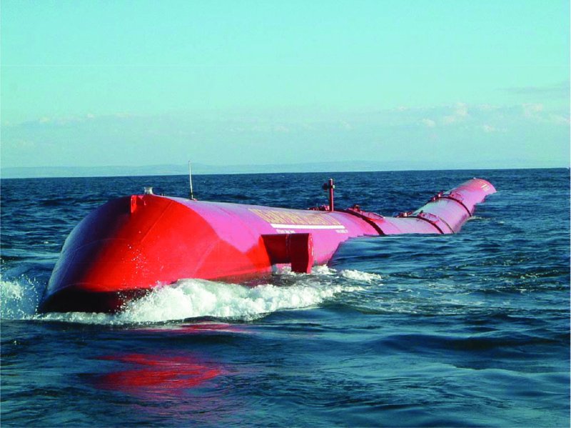
Figure 7.30 The Pelamis wave energy converter at sea. Courtesy of Umanji Solar. http://buildipedia.com/aec-pros/public-infrastructure/pelamis-wave-energy-converter-renewable-energy-from-ocean-waves
7.3 Tidal power
The daily rising and falling of the sea level is a familiar sight. Close to a coastline, the difference in height between low tide and high tide, called the range, can be considerable, ∼ several metres or more. Clearly this involves huge changes in the potential energy of the water. If the water at high tide is trapped behind a dam or barrier, this potential energy can be harnessed in an analogous way to a hydroelectric plant. Tides may also result in the flow of water through narrow channels that connect large areas of water. Such channels occur, for example, between the mainland and a nearby island. These tidal currents may reach speeds of ∼5 m/s and provide an alternative way to harvest tidal power. This power can be harnessed in a similar manner to the way wind turbines harness wind power although, of course, the water turbines are located under water.
We remark straight away that tidal motions are complicated and so are difficult to predict. This is not least because of the topography of a particular location, for example the shape of the seabed close to a coastline or the occurrence of estuaries or bays. However, detailed observations have been made of tidal motion over many decades at many locations because knowledge of local tides is essential for the navigation of shipping. And it is these long-term observations that are the basis upon which tide motion can now be successfully predicted. Thus any variations in output power from a tidal power plant can be foreseen and taken into account when delivering power to a national grid. Tidal power has other important advantages. It is a renewable energy source and it has the potential to deliver enormous amounts of energy. It is estimated that the sites of greatest potential throughout the world could provide ∼120 GW of power and that, in principle, 25% of the UK's energy needs could be supplied by tidal power. The main drawback of tidal power has to do with the very high costs involved in building the power plants. Moreover, the sites for these plants have very specific requirements with regard to their topography, and the availability of suitable sites is limited. An additional issue is the large ecological impact that a tidal power plant has on the local environment. For these reasons, only a few tidal power plants have been constructed so far. However, further plants are being proposed including one to be sited in the Bristol Channel, UK. In this section we present simplified models to describe the origin and behaviour of the tides. We also describe ways in which tidal power can be harnessed.
7.3.1 Origin of the tides
It is well known that the tides are caused by gravitational forces that the Moon and Sun exert on the Earth and its oceans. Indeed the link between the tides and the motion of the Moon was recognised in ancient times. But why does the Moon play the dominant role even though the Sun's gravity is almost 200 times greater? And why are there two tides each day? It was Newton who first successfully described the origin of the tides in his Principia and it was a great victory for his universal law of gravity to provide the answers to these questions. Since then, many scientists have contributed to a more detailed understanding of tidal motions, including George Airy, Pierre-Simon Laplace, George Darwin (son of Charles Darwin) and Lord Kelvin.
The gravitation force between two spheres is the same as if the mass of the each sphere were concentrated at its centre. However, the gravitational force exerted by sphere A upon sphere B is not constant over the surface of sphere B. So, the occurrence of the tides is not simply the gravitational attraction of the Moon and the Sun; the tides result from the way in which the gravitational attraction of the Moon and the Sun vary over the surface of the Earth. All particles on Earth are attracted to the Moon and Sun by gravity, but some are attracted more and some are attracted less, depending on their location.
Figure 7.31 shows schematically the Earth–Moon system, as it is the Moon that dominates tidal motion. The Earth and the Moon mutually attract each other as described by the universal law of gravity. The gravitational pull on the water on the near side to the Moon is greater than the gravitational pull on the Earth because it is closer to the Moon. Because the water is fluid, it flows to produce a bulge of water on the side facing the Moon. The gravitational pull on the water on the far side of the Earth is less than the gravitational pull on the Earth and so water flows to produce a bulge of water on that side too. It is not that the water is pushed away from the Moon, but that the gravitational pull is less. Then as the Earth revolves about its axis, a given geographical location on Earth, say point P in Figure 7.31, experiences two high tides and two low tides each day.
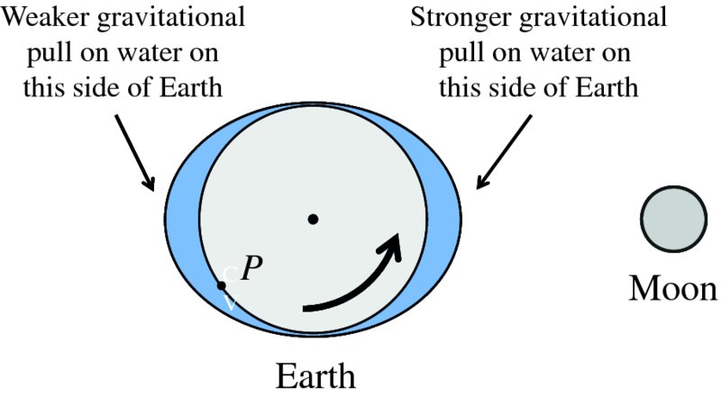
Figure 7.31 The Earth and the Moon mutually attract each other as described by the universal law of gravity. The gravitational pull on the water on the side facing the Moon is greater than the gravitational pull on the Earth because it is closer to the Moon. As the water is fluid, it flows to produce a bulge of water on the side facing the Moon. The gravitational pull on the water on the far side of the Earth is less than the gravitational pull on the Earth and so water flows to produce a bulge of water on that side too. Then as the Earth revolves about its axis, a given geographical location on Earth, say point P, experiences two high tides and two low tides each day.
To be more quantitative about the variation in the gravitational pull of the Moon, we consider its gravitational attraction on two identical particles of mass m that are on opposite sides of Earth, as illustrated in Figure 7.32. We are only interested in the gravitational attraction of the Moon on these two particles and so we ignore the gravitational attraction that the Earth exerts on them. Mass m is small, say 1 kg, and so the gravitational force of attraction between the two particles can also be ignored. The Moon's gravitational force of attraction FA on the particle at point A is given by
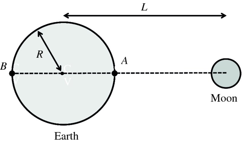
Figure 7.32 A particle on the side of the Earth closest to the Moon experiences a larger gravitational force of attraction from the Moon than an identical particle on the far-side. The difference in these gravitational forces depends on the cube of the distance L.
where G is the gravitational constant, MMoon is the mass of the Moon, R is the radius of the Earth and L is the distance between the centres of the Earth and the Moon. The gravitational force of attraction FB of the Moon on the particle at point B is given by
The difference between the two is
which we can write as
As R ≪ L, this reduces to

We see that the difference in the Moon's gravitational attraction on the two particles depends on the cube of the distance L. This inverse-cubic dependence on distance rather than the more familiar inverse-square dependence arises because we are dealing with a difference between two forces. The inverse-cubic dependence explains why the Moon has a greater influence on the tides than the Sun. Although the Sun is much more massive than the Moon, the variation in its gravitational field across the Earth is smaller.
Tidal force
We have seen that the gravitational force of the Moon is not constant over the surface of the Earth, the nearest side is attracted more strongly than the furthest side. Such differences in gravitational attraction give rise to the so-called tidal force. The tidal force is not of itself a force but rather it is a differential force, being the difference between the gravitational force acting at different locations. It is the tidal force that is responsible for the tides. For our discussion of the tides, we define the tidal force acting on a particle at a given location as the vector difference between the gravitational force acting on the particle and the gravitational force acting on an identical particle located at the Earth's centre.
We can explain this result as follows. For a particle located at the centre of the Earth, the Moon's gravitational force of attraction is exactly balanced by the centrifugal force the particle experiences. Hence there is no net force tending to pull or push the particle away from this location. All identical particles on or in the Earth experience the same centrifugal force; the same in magnitude and the same in direction. This direction lies parallel to the line connecting the Earth and Moon centres. However, the Moon's gravitational force of attraction varies over the Earth. Consequently, for particles at locations other than the Earth's centre, the Moon's gravitational pull is not balanced by the centrifugal force with the result that the particle will experience a net force that pushes or pulls it. The net force is the vector addition of the centrifugal force and Moon's gravitational force of attraction. Those particles that can move will do so and consequently the waters of the Earth flow to produce the tidal bulges. Since the centrifugal force and the gravitational force acting on a particle at the Earth's centre are equal and opposite, it follows that the net force, i.e. the tidal force, experienced by an identical particle anywhere else is equal to the vector difference between the gravitational force it experiences and the gravitational force experienced by the particle at the Earth's centre. We now use this result to deduce the tidal force at different locations on Earth and we will see how the waters of the Earth move under the influence of the tidal force to produce the two tidal bulges we see in Figure 7.31.
Figure 7.33 shows the positions of three identical particles, one at the Earth's centre and the others at points A and B on opposite sides of the Earth. The gravitational forces, FO, FA and FB, that act on these particles are represented by black arrows. These arrows point towards the centre of the Moon, of course. The arrow at point A is longer than the one at point B, indicating the relative magnitudes of the two forces. The particle at the centre of the Earth experiences an attractive force of magnitude FO, which is essentially the mean of the magnitudes of the forces at points A and B, a result we can readily obtain using the previous analysis. The tidal force acting on the particle at A is the vector difference between FO and FA, as indicated by the figure; this tidal force is shown as a blue arrow on Figure 7.33. We see that tidal force at A points away from the Earth's centre. The same procedure gives the tidal force at B, which is also represented by a blue arrow. At that point, the tidal force again points away from the Earth's centre.
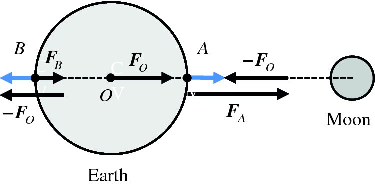
Figure 7.33 The figure shows the positions of three identical particles, one at the Earth's centre and the others at points A and B on opposite sides of the Earth. The Moon's gravitational forces, F0, FA and FB, that act on these particles are represented by black arrows. The tidal force acting on a particle at a given point is equal to the vector difference between the gravitational force exerted on the particle and the gravitational force, F0, exerted on an identical particle at the Earth's centre. The resulting tidal forces at points A and B are indicated by the blue arrows and point away from Earth's centre.
We can extend this procedure to obtain the tidal force at an arbitrary point P on the Earth's surface. For this we adopt the representation shown in Figure 7.34. In this representation, point P has coordinates (x, y), with x = Rcos θ and y = Rsin θ with respect to the Earth's centre. Again we compare the Moon's force of attraction on identical particles at P and at the Earth's centre. The magnitude FO of the gravitation force on a particle at the centre of the Earth is given by
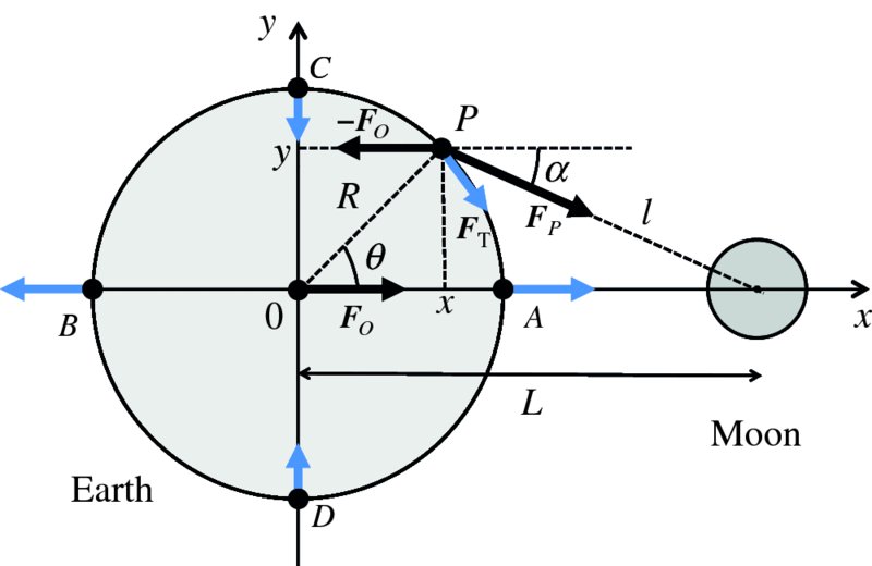
Figure 7.34 The figure shows the construction to obtain the tidal force acting on a particle at an arbitrary point P on the Earth's surface. FP is the gravitational force acting on the particle, while FO is the gravitational force acting on a particle at the Earth's centre. The blue arrow represents the resultant tidal force FT.
where m is the mass of the particle. The magnitude FP of the gravitation force, on the particle at P is given by
where l is the distance of P to the Moon's centre. The component of this force in the x-direction is
where the angle α is defined in Figure 7.34. Hence the tidal force FT at P has a component FT,x in the x-direction that is given by
We have
since L ≈ l and x ≪ l. Hence,

This rearranges to give:
as
 ≪
≪
 . Then, because x ≪ L, we can write
Substituting for l2 in Equation (7.103), we obtain

The y-component of the gravitation force FP on the particle at P is
The gravitational force FO acting on the particle at the Earth's centre has no component in the y-direction and so the y-component of the tidal force at P is simply given by
As sinα is very small,
 . Hence, taking l ≈ L, we obtain
Hence the x- and y-components of the tidal force at point P are given by

within the approximations we have made.
At point A on Figure 7.34, θ = 0. Hence,
Thus the magnitude of the tidal force is
and the force points away from the Earth's centre, as represented by the blue arrow at that point. At point B, with θ = π, the magnitude of the tidal force is also

and again the force points away from the Earth's centre, as cos (π) = −1. At point C, θ = π/2. Hence, FT, x = 0 and
We see that the tidal force has a magnitude that is half its value at A and B and is directed inwards. At point D,
 . The tidal force has the same magnitude as at C, but points in the opposite direction, again directed inwards.
Using Equations (7.105) and (7.108), we can obtain the strength and direction of the tidal force for all positions on the surface of the Earth. When we do this we obtain the diagram shown in Figure 7.35, where the blue arrows indicate the relative magnitude and direction of the tidal force at various places on the Earth's surface.
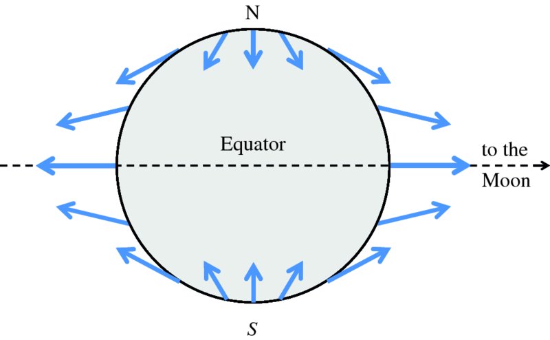
Figure 7.35 The blue arrows represent the direction and relative strength of the tidal force at various places on the Earth's surface.
We model the Earth as a sphere of solid matter that is covered by a relatively thin layer of water; the average depth of water in the oceans is ∼4000 m, which is less than 1% of the Earth's radius. The tidal force has relatively little effect on the solid Earth, but the water can readily flow under the influence of the force. The tidal force, illustrated by the blue arrows in Figure 7.35, has a component parallel to the Earth's surface and a component normal to the surface. It is the parallel component that produces the tidal bulges. This component ‘pushes’ the water towards either side of the Earth, forming the two water bulges seen in Figure 7.31. The perpendicular component of the tidal force has little effect on the water. We can see this as follows. From Equations (7.105) and (7.108), the strength of the tidal force FT on a particle of mass m is
while the strength of the gravitational force Fg on an identical particle at the Earth's surface is
Hence, their relative strengths are given by
Putting in appropriate values:
We see that the tidal force is far too weak compared with the Earth's gravitational attraction for it to ‘raise’ the level of the oceans. On the other hand, the Earth's gravitation force does not have a component parallel to the Earth’ s surface and so the parallel component of the tidal force is effective in creating the water bulges.
The reader may expect tidal forces to distort the shape of the solid Earth: to stretch the planet along the line connecting the Earth and Moon. They do, but because of the Earth's rigidity, the extent of such distortions is small compared with the tidal range of an ocean. The reader may also expect that the rotation of the Earth about its own axis would cause it to bulge around the equator. It does. In fact the Earth is described as an oblate spheroid, where the distance from Earth's centre to sea level is about 20 km greater at the equator, the polar radius being approximately 0.3% shorter than the equatorial radius. However this is a constant effect that is independent of the motion of the Moon or Sun. It simply forms the underlying shape of the Earth's surface upon which the oceans move.
Apart from being responsible for the Earth's tides, tidal forces also arise in many astronomical situations. Their effects are evident where the gravitational force of attraction due to a large body varies across the spatial extent of another body, causing that body to become distorted in shape or even to pull apart. A particular example is a moon of Jupiter called Io. The mass of Jupiter is more than 300 times the mass of Earth and it exerts a correspondingly large gravitational pull. Io is the moon of Jupiter that lies closest to the planet. Jupiter, in conjunction with its other moons, exerts huge tidal forces on Io, causing it to be continuously distorted, rather like a squash ball being rapidly squeezed and released. These deformations generate friction and enough heat to give Io a molten interior. As a result, molten lava spews out of numerous volcanoes on its surface, making Io the most volcanically active world in the solar system. This volcanic activity was revealed by the high-resolution images of Io received from the Voyager spacecraft in 1979. The gravitational pull of Jupiter also led to the break-up of comet Shoemaker-Levy 9. In 1992, the comet passed close to Jupiter and the tidal force exerted by the planet on the comet caused it to pull apart into more than 20 fragments. Then in 1994, these fragments spectacularly collided with Jupiter, providing the first direct observation of an extraterrestrial collision of solar-system objects.
Period of lunar tides
We have seen that at most geographical locations there are two high tides each day. This suggests that high tides are separated by 12 hr. In fact they are separated by 12 hr 25 min. This is because, as well as the Earth rotating about its own axis, the Moon moves in its orbit around the Earth. This is illustrated schematically in Figure 7.36, which is the view of the Earth–Moon system from Polaris, the north star. From this direction the Earth rotates about its own axis in an anti-clockwise direction, while the Moon orbits the Earth also in an anti-clockwise direction. The figure shows two positions of the Moon, A and B. Initially point P on Earth is directly below the Moon, which is at position A. After one full revolution of the Earth about its axis, which takes 24 hr, the Moon has moved from A to B. Then it takes the Earth about 50 minutes to catch up with the Moon so that point P is once again directly ‘under’ the Moon. As there are two high tides per day, it follows that they are separated by approximately 12 hr 25 min.

Figure 7.36 This figure shows the view of the Earth–Moon system from Polaris, the north star. From this direction the Earth rotates about its axis in an anti-clockwise direction, while the Moon orbits the Earth also in an anti-clockwise direction. Initially, point P on earth is directly below the Moon, which is at position A. After one full revolution of the Earth about its axis, the Moon has moved from A to B. So the Earth must then rotate a further amount until point P is once again directly ‘under’ the Moon. It takes the Earth about 50 minutes to catch up with the Moon.
7.3.2 Variation and enhancement of tidal range
At the beginning of our discussion of the tides, we emphasised that tidal motions are complicated. Not surprisingly the tidal range at a particular location is invariably very different from that predicted for the middle of an ocean. Indeed, the tidal range at a coastal location may be an order of magnitude or more larger, say ∼5m. There are various additional factors that may affect tidal range. These include:
- the Moon is not usually in the equatorial plane of the Earth;
- the Sun's gravitational attraction, which we have so far neglected, also influences the tides;
- the tidal bulges do not align with the Earth–Moon axis;
- the topography of the coastal location – this is usually the most important factor of all.
We deal with these factors in turn. So far it has been convenient to assume that the Moon is situated directly above the Earth's equator. However, this is usually not the case. Firstly the orbit of the Moon is inclined at an angle of 5° with respect to the Earth's equatorial plane – the plane of the Earth's orbit about the Sun. And more importantly, the axis of the Earth's daily rotation is inclined at an angle of 23.5° with respect to its equatorial plane. In Section 4.3.2 we considered how the inclination of the Earth's axis leads to the occurrence of the seasons (see Figure 4.15). We defined the Sun's angle of declination as the angle between the Earth's equatorial plane and a line drawn from the centre of the Earth to the centre of the Sun. We saw how this angle varied from + 23.5° at the summer solstice to − 23.5° at the winter solstice. Similarly, the Moon has an angle of declination δ with respect to the Earth's equatorial plane, which changes continuously as it orbits the Earth. If, for the sake of simplicity, we neglect the relatively small angle that the Moon's orbit makes with the Earth's orbit, the angle δ varies continuously from + 23.5° to − 23.5° during the ∼28 day cycle of the Moon's orbit.
Figure 7.37 shows the Earth–Moon system when δ has a positive value and when the Moon is directly above the equator, with δ = 0. The figure also compares the orientations of the tidal bulges for these two cases; the tidal bulges have been greatly exaggerated for the sake of clarity. As δ increases, the tidal bulges move to follow the Moon and are no longer aligned with the Earth's equator. Then, as we can see from the figure, the two high tides at latitude P will have different heights. Furthermore, at high latitudes such as at Q, there will be only one tide rather than two. An analogous situation occurs for negative values of δ.
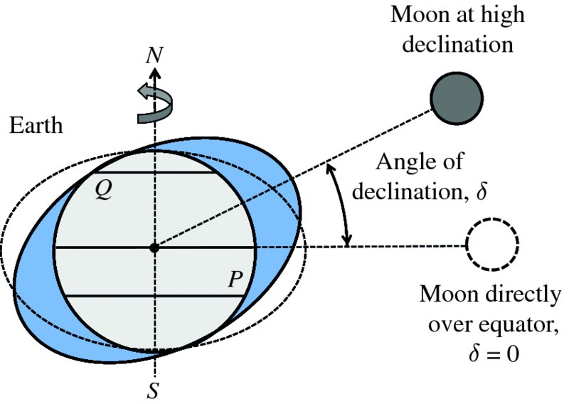
Figure 7.37 This figure shows the Earth–Moon system when the moon's angle of declination δ has a positive value and when the Moon is directly above the equator, with δ = 0. The figure also compares the orientations of the tidal bulges for these two cases; the tidal bulges have been greatly exaggerated for the sake of clarity. As δ increases, the tidal bulges move to follow the Moon and no longer align with the Earth's equator. From the figure we can see that the two high tides at latitude P will have different heights. Furthermore, at high latitudes such as at Q, there will be only one tide rather than two.
The gravitational influence of the Sun on the tides is less than half as strong as that of the Moon, as we have seen, but the Sun still plays a significant role in determining tidal range. We can see this pictorially in Figure 7.38, which is a view of the Sun–Earth–Moon system from Polaris. When the Moon is line with the Sun, at positions A or B, the gravitational pull of the Sun enhances the gravitational pull of the Moon. At these times the tidal range is greatest and the tides are called spring tides. When the Moon is on a line that is perpendicular to the direction of the Sun, at positions C or D, the gravitational pull of the Sun and of the Moon act in different directions. The effect of this is to reduce the tidal range and such tides are called neap tides. Figure 7.38 also shows the corresponding phases of the Moon.
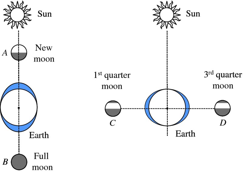
Figure 7.38 When the Moon is in line with the Sun, at positions A and B, the gravitational pull of the Sun enhances the gravitational pull of the Moon. At these times, the tidal range is greatest and the tides are called spring tides. When the Moon is on a line that is perpendicular to the direction of the Sun, at positions C and D, the gravitational pull of the Sun and of the Moon act in different directions. The effect of this is to reduce the tidal range and such tides are called neap tides. The figure shows the corresponding phases of the Moon.
The model of the tides that we described in Section 7.3.1 is called the equilibrium tide model. In this model we have tidal bulges either side of the Earth, which are fairly static since the Moon takes a month to revolve about the Earth, and the Earth rotates within these tidal bulges. From a different viewpoint, we can think of ocean tides as a dynamic system. From this viewpoint, the Moon produces a periodic force that drives the oceans to and fro between the continents. We may recall the familiar example of a forced oscillator of a mass on a spring that is driven by a periodic force. In general there is a phase difference between the displacement of the mass and the driving force. So it is with the tides. In reality the tidal bulges are not aligned with the Earth–Moon axis as shown in Figure 7.39. There is a phase lag between the peak of the bulge and the ‘overhead’ position of the Moon.
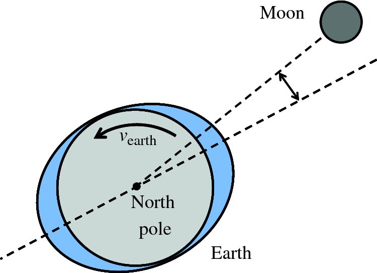
Figure 7.39 In reality, the tidal bulges are not aligned with the Earth–Moon axis. There is a phase lag between the peak of the bulge and the ‘overhead’ position of the Moon because the tidal bulge cannot move quickly enough to keep up with the motion of the Moon.
We can get some physical insight into the dynamic behaviour of the tides by considering the tidal bulge to behave like a water wave as it moves across the oceans and indeed it is called a tidal wave. (This is the correct meaning of the term tidal wave; Tsunamis are generated by abrupt movements in the Earth's surface layer and are not tidal waves, although they are often described in this way.) For the tidal bulge to remain directly below the Moon, the bulge would have to travel at the same speed as the surface of the Earth that rotates beneath it. However, the tidal bulge cannot move fast enough to achieve this. Taking the Earth to rotate once on its axis in 24 hr and the radius of the Earth to be 6400 km we find the linear velocity of a point on the Earth's equator to be
We can assume here that the Moon is stationary since it takes about 28 days to orbit the Earth. In Section 7.2.2, we found that the group velocity of a shallow water wave is given by
where g is the acceleration due to gravity and h0 is the depth of the water. By shallow we mean that the wavelength λ of the wave is
long compared with the water depth h0. The average depth of the world's oceans at about 4000 m certainly cannot be called
shallow, but the wavelength of the tidal bulge is much larger than this; in principle
its wavelength is about half the circumference of the Earth. Thus the requirement
λ ≫ h0 is obtained. Thus, according to Equation (7.90), the velocity of the tidal bulge
is ∼
 m/s, i.e. about 200 m/s (∼700 km/hr). This is much less than the velocity of the
Earth's surface and the tidal wave cannot keep up with the Earth's rotation. The picture
we thus obtain is as shown in Figure 7.39; there is a time lag between the peak of
the bulge and the Moon's position. We also note that as a tidal wave propagates across
an ocean, it experiences a Coriolis force, just as the global winds do. The tidal waves are similarly
deflected and indeed tidal waves are observed to follow circular patterns on a global
scale.
m/s, i.e. about 200 m/s (∼700 km/hr). This is much less than the velocity of the
Earth's surface and the tidal wave cannot keep up with the Earth's rotation. The picture
we thus obtain is as shown in Figure 7.39; there is a time lag between the peak of
the bulge and the Moon's position. We also note that as a tidal wave propagates across
an ocean, it experiences a Coriolis force, just as the global winds do. The tidal waves are similarly
deflected and indeed tidal waves are observed to follow circular patterns on a global
scale.
In reality, the topography of a particular coastline is usually the dominant factor in determining tidal range. Close to coastlines, the water depth usually decreases significantly. When the tidal wave runs into shallow waters, its velocity is reduced (see Equation 7.90). Then the energy of the wave accumulates in a smaller volume and the rise and fall of the tide are amplified. In addition, estuaries and bays can have a particularly large effect on tidal range. They funnel the incoming tide and thus greatly amplify tidal range. As we saw in Section 7.2.3, such an effect is exploited in an overtopping power plant.
There may also be resonant enhancement of the tidal range in a bay or an estuary. When we push a playground swing, we time the pushes so that they match the natural frequency of the swing. At this resonance frequency a small effort causes a large amplitude of swing. The rising and falling tide at the entrance to a bay acts as a driving force that causes the body of water within the bay to rise and fall. The body of water also has a resonant frequency. If the frequency of the driving tide is close to this resonant frequency, a standing wave is set up in the bay and this amplifies the tidal range. If we swing a bucket of water to and fro, the water also sloshes to and fro and, in particular, the water rises abruptly at the sides of the bucket. Similarly, in the resonant enhancement of the tides in a bay, the maximum tidal range occurs at the closed end of the bay.
A simple model of a bay is shown in Figure 7.40, where the bay has length L. The tidal motion at the entrance to the bay sets up a standing wave of water with
wavelength λ. The first resonant mode in the bay occurs for
 , as illustrated in Figure 7.40, where the blue dotted curve represents the elevation
of the water in the bay. The period T of the resulting standing wave is given by
, as illustrated in Figure 7.40, where the blue dotted curve represents the elevation
of the water in the bay. The period T of the resulting standing wave is given by

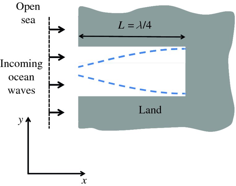
Figure 7.40 The figure shows a simple model of a bay. The rising and falling tide at the entrance to the bay acts as periodic driving force that causes the body of water within the bay to rise and fall. The body of water also has a resonant frequency. If the frequency of the driving tide (∼12.5 hr) is close to this resonant frequency, a standing wave of water is set up in the bay and this amplifies the tidal range. The first resonant mode in the bay occurs for L = λ/4, where λ is the wavelength of the standing wave. The blue dashed curves represents the elevation of the water in the bay at resonance. Maximum elevation is obtained at the closed end of the bay.
where v is the wave velocity. As the water in a bay is usually shallow, we can take the wave
velocity to be given by
 (Equation 7.90). Hence,

Resonance enhancement occurs when the period of the tide in the open sea matches the period, T, of this resonant mode. Of course, real estuaries and bays do not have the uniform dimensions of our simple model. However, the Bay of Fundy, New Brunswick, Canada, has a shape that is not too dissimilar to that shown in Figure 7.40. The length of the Bay of Fundy is ∼300 km and the average depth is ∼70 m. Using these values of L and h0, respectively, we find that the value of the period T for the bay is
This period is close to the period ∼12.5 hr at which the Moon drives the tides – the time between high tides in the North Atlantic. Consequently, the Bay of Fundy has a tidal range that exceeds 15 m at some times in the year, the highest tidal range in the world. This value can be compared with the typical tidal range in open ocean, which is ∼0.5 m.
An example of the variation of tidal range over the period of a month is shown in Figure 7.41. It was recorded at Bridgeport, Connecticut, USA. The sea level rises and falls in a sinusoidal-like fashion with a period of ∼12.5 hr, due to the Earth's rotation. The tidal range varies over the course of the month due to the relative motions of the Moon and Sun, giving rise to two spring tides and two neap tides per month. In this example, the tidal range of the spring tides is about twice as large as that of the neap tides, which is quite typical.
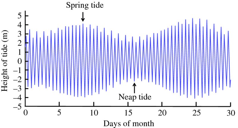
Figure 7.41 An example of the variation of tidal range over the period of a month, which was recorded at Bridgeport, Connecticut, USA. The sea level rises and falls in a sinusoidal-like fashion with a period of ∼12.5 hr, due to the Earth's rotation. The tidal range varies over the course of the month due to the relative motions of the Moon and Sun, giving rise to two spring tides and two neap tides per month.
7.3.3 Harnessing tidal power
There are two main ways in which tidal power is harnessed. One exploits the potential energy of water at high tide and is called tidal range power. The other exploits the kinetic energy of tidal water that flows through narrow channels and is called tidal current power.
Tidal range power
The principle of operation of a tidal range power plant is similar to that of a hydroelectric plant. A barrier is built across the mouth of an estuary or bay, thus forming a reservoir behind the barrier. As the sea level rises with the high tide, water is allowed to pass into the reservoir through a sluice gate. When high tide is reached the sluice gate is closed, trapping water at the high-tide level in the reservoir. Then when the sea level drops at low tide, the trapped water is passed through a turbine, which is connected to an electrical generator. In contrast to a conventional hydroelectric plant, the head of water is low ∼5 m and the water flow rate is high, and the turbines must be designed to take this into account.
If the surface area of the tide pool containing the collected water is A and the tidal range is D then the potential energy U of the stored water is given by
where ρ is the density of seawater and g is the acceleration due to gravity. The factor of ½ arises because the centre of
mass of the body of water falls through distance ½D. The quadratic dependence on D emphasises the importance of having as large a value of D as possible. The average power
 is then given by

where τ is the tidal period. As we have seen, tidal range, and hence the available power, varies throughout the month and year and an approximation that is used for the average power is
where
 is the mean range of all tides. Taking
 , A = 10 km2, ρ = 1.03 × 10³ kg/m3, g = 9.8 m/s2 and τ = 12 hr 25min = 4.47 × 10⁴ s, we obtain

As usual, the maximum possible power cannot be achieved in practice and the overall efficiency of the system for producing electricity may be ∼80% of this value.
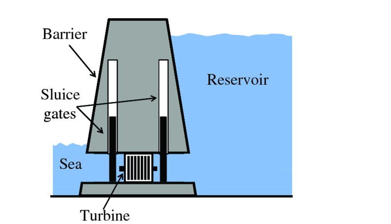
Figure 7.42 A schematic diagram of a tidal range power plant. By suitable manipulation of the sluice gates, the turbine is driven by water that flows into the reservoir as well as by water that flows out as the tide rises and falls.
The output tidal range power can be doubled if the plant uses reversible turbines that are driven by water that flows into the reservoir as well as by water that flows out. The arrangement for this is illustrated in Figure 7.42, where the barrier contains two sluice gates. The cycle of events is as follows. Let us say that the water level in the reservoir is initially at the high-tide level and that the tide is low on the sea side. The sluice gates are opened and water from the reservoir flows through the turbine. Then when the water level in the reservoir has fallen to low-tide level, the sluice gates are closed. After low tide has been reached, the sea level steadily rises to high-tide level, high above the water level in the reservoir. When high tide is reached, the sluice gates are opened and water flows through the turbines from the sea to the reservoir. The reservoir steadily fills up and when high-tide level is reached, the sluice gates are closed. The cycle then repeats.
A notable example of a tidal range plant is the Rance Tidal Power Station that is located on the estuary of the Rance River in Brittany, France, where the average tidal range is a massive 8 m, the highest in France. It was opened in 1966 as the world's first tidal range power station and was for 45 years the largest such power station, until the South Korean Sihwa Lake Tidal Power Station was opened in 2011. The Rance tidal basin has a total area of 22.5 km2. Its power station has 24 turbines and they produce a peak output power of 240 MW and an average power of 62 MW. A photograph of the Rance Tidal Power Station is shown in Figure 7.43.
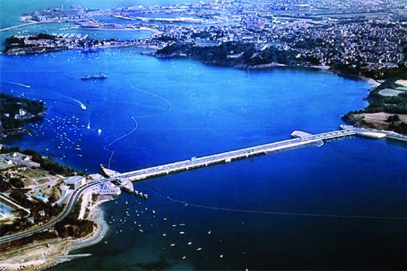
Figure 7.43 A photograph of the Rance Tidal Power Station which is located on the estuary of the Rance River in Brittany, France, where the average tidal range is a massive 8 m. The Rance tidal basin has a total area of 22.5 km2, and the power station has 24 turbines which produce a peak output power of 240 MW and an average power of 62 MW. Source: http://theearthproject.com/wp-content/uploads/2016/01/La-Rance-Tidal-Power-Plant.jpg
Tidal current power
As previously noted, tides can also result in the flow of water through narrow channels that connect large areas of water, for example a channel between the mainland and a nearby island. Moreover, these tidal currents may reach speeds of ∼5 m/s. Energy can be harvested from the flowing water just as energy is harvested from the wind; the water is passed through turbines that drive electrical generators. The potential power, P, from a water turbine is described by the same equation as for a wind turbine (see Equation 6.15):
where A is the area of the turbine, ρ is the density of seawater and v is the velocity of the water. The important difference between water and wind turbines is that the density of water is about 800 times greater than that of air. This higher density compensates for the fact that water velocities are generally smaller than wind velocities. And a water turbine is immersed in seawater, which is a harsh environment. Taking a turbine diameter of 15 m, a water velocity of 3.0 m/s and a seawater density of 1.03 × 10³ kg/m3, we obtain
which is of the same order as the power from a wind turbine.
An important example of a tidal current power plant is called SeaGen, which was installed in Strangford Lough in Northern Ireland in 2008. One of the principal features of this lough is a restricted channel that connects it to the Irish Sea and through which seawater flows in and out of the lough. The channel is ∼8 km long, with a minimum width of ∼1 km and a depth varying between 30 and 60 m. This constriction results in very strong currents that peak in excess of 4.5 m/s on spring tides and it is estimated that ∼3.5 × 10⁸ m3 of water enters and leaves the lough at each tide. Interestingly, it is recorded that Strangford Lough was exploited as a tidal energy source as far back as 532 AD, when a tidal mill was used as part of a monastic settlement.
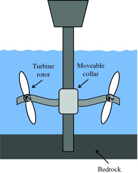
Figure 7.44 A schematic diagram of the SeaGen tidal current plant at Strangford Lough in Northern Ireland. The rotor diameter of each turbine is 16 m and each turbine drives a generator. The turbines have a feature that allows them to operate for water flowing into or out of the lough. The crossbeam is attached to a collar which slides over a central column. This allows the turbines to be lifted above the water line for routine maintenance.
A schematic diagram of the SeaGen plant is shown in Figure 7.44. It consists of twin turbines mounted on a crossbeam. The rotor diameter of each turbine is 16 m and each turbine drives a generator. The turbines have a patented feature that allows the rotor blades to be pitched through more than 180°. This allows the turbines to operate for water flowing into or out of the lough. The crossbeam is attached to a collar that slides over a central column and this allows the turbines to be lifted above the water line for routine maintenance. At full power, SeaGen delivers a maximum power of 1.2 MW and delivers up to 20 MWh/day. Currently, the SeaGen plant is the only commercial tidal current plant in the world, although similar plants are planned for other locations.
Problems 7
-
A transverse wave travelling along a taut string is described by the function y = 25cos (0.15x + 75t), where x and y are in millimetres and t is in seconds. (a) Find (i) the amplitude, (ii) the wavelength, (iii) the frequency (Hz), and (iv) the velocity of the wave. In what direction is the wave travelling? (b) What is the maximum transverse velocity and acceleration of an element of the string?
-
One end of a long taut string is moved up and down in simple harmonic motion with an amplitude of 0.10 m and a frequency of 10 Hz. At time t = 0, the end of the string (at x = 0) has its maximum upward displacement. The resultant wave travels down the string in the positive x-direction with velocity 40 m/s. Obtain an equation describing the wave.
-
You move one end of a long rope in simple harmonic motion with amplitude 0.15 m and frequency 4.0 Hz, while maintaining a tension of 50 N in the rope. The other end of the rope is connected to a distant tree. The rope has a mass of 0.5 kg/m. (a) How much energy is contained in a length of the rope equal to one wavelength of the transmitted wave? (b) How much power are you expending? (c) What will be the required power if: (i) the frequency is doubled; (ii) the amplitude is halved?
-
Show that y = Asin (ωt − kx) + Bsin (ωt + kx) is a solution of the one-dimensional wave equation.
-
The Glendoe hydroelectric plant in Scotland has a catchment area for rainfall of 75 km2, and the annual rainfall is approximately 2 m. The plant has a head of 600 m, the highest in the UK. Make an estimate of the average power that this plant can provide.
-
The flow of liquid through a pipe depends on: (i) the coefficient of viscosity η; (ii) the radius a of the pipe; and (iii) the pressure gradient g set up along the pipe. The pressure gradient is
 , where p is the pressure difference between the ends of the pipe and l is its length. Use the method of dimensions to find an expression for the flow rate
in terms of η, a, and g, and then in terms of η, a, p and l. Note that the units of η are Ns/m2.
, where p is the pressure difference between the ends of the pipe and l is its length. Use the method of dimensions to find an expression for the flow rate
in terms of η, a, and g, and then in terms of η, a, p and l. Note that the units of η are Ns/m2.
-
Compare the difference in the gravitational pull of the Earth at the nearest and furthest sides of the Moon with the difference in the gravitational pull of the Moon at the nearest and furthest sides of the Earth.
-
Show that the latitude on Earth at which the tidal force due to the Moon is parallel to the Earth's surface is 54.7°, i.e. the latitude at which the vertical component of the tidal force is zero.
-
(a) Calculate the distance of the centre of mass of the Earth–Moon system from the Earth's centre as a fraction of the Earth's radius. (b) Calculate the distance of the centre of mass of the Sun–Earth system from the Sun's centre as a fraction of the Sun's radius. The masses of the Earth, Moon and Sun are 5.97 × 1024 kg, 7.35 × 10²² kg and 1.99 × 1030 kg, respectively; the distance between the Earth and Moon is 3.84 × 10⁵ km and that between the Sun and Earth is 1.50 × 10⁸ km; the radii of the Earth and Sun are 6.38 × 10³ km and 6.96 × 10⁵ km, respectively.
-
For waves on deep water, the angular frequency ω and wavenumber k are related by the dispersion relation
where g is the acceleration due to gravity, and ρ and S are the density and surface tension of the liquid, respectively. Determine the minimum value of the phase velocity for water waves on deep water. The density and surface tension of water are 1.0 × 10³ kg/m3 and 7.2 × 10− 2 N/m. Assume g = 9.8 m/s2.
-
For a canal 4.0 m deep, calculate the phase velocity and group velocity for water waves of wavelength (i) 10 mm, (ii) 1.0 m and (iii) 50 m.
-
The British Isles has about 1000 km of Atlantic coastline. Calculate the average wave power that this could provide, assuming the amplitude, H, of the waves is 1.0 m and the group velocity vg is 8.0 m/s. Assuming 50% of this could be converted into electrical power, approximately how much electrical power would be provided per person in the British Isles?
-
A tidal power plant utilising the incoming and outgoing tides has a tide pool of area 22.5 km. Taking the average tidal range to be 8 m, calculate the maximum possible output power of the plant. Calculate the power per square metre of the tide pool. How does this energy density compare with the same quantity for a wind farm? How large must the tide pool be for the generation of 2.5 MW? Take the density of seawater to be 1030 kg/m3.
-
Suppose that we build a water farm of underwater turbines in the Irish Sea. What power per square metre of the sea should we obtain? Assume that the underwater turbines must be separated in the same way that wind turbines are separated on land. Take the average speed of the water to be 1.0 m/s and assume an overall efficiency of 50%.