In this section, we will simulate a quantum circuit using Python. The good news is that it's easy, as we've already done it. A quantum circuit is merely a sequence of quantum gates. One example is Y |"+">, another example is XH|"0">. In the circuits we work with on IBM QX, the initial state will always be |"0"> for a given qubit.
A quantum circuit diagram is a method to visualize quantum circuits. Typically, on the left-hand side of a quantum circuit diagram, we'll start with a series of |"0"> qubits with lines coming out of them that look a bit like wires; hence the name quantum circuits. Quantum gates can be placed along the lines in the order they are to be applied to the |"0"> qubit, with their name and a box drawn around it. For multiqubit-controlled gates, such as CNOT, the gate is put on the target qubit wire, and a line is drawn from the gate to the control qubit wire. The target qubit has a larger, open circle drawn around it, while the control qubit has a smaller black circle drawn on it.
When we write gates in words/algebra or in code, we put |"0"> on the right side, as in XYZ|"0">, and apply the gate closest to the qubit first, going from right to left. This is an artifact of the mathematical operations underlying the gate application. With quantum circuits, we have a setup that is more like reading in English. We go from left to right, applying gates in the order that we read them to the |"0"> qubit. From now on, we'll primarily deal with visual quantum circuits as we program! So, just remember, in a quantum circuit things go from left-to-right, but in a Python program or words/algebra, things go from right-to-left.
Let's first look at some quantum circuit diagrams for quantum circuits we have already seen in previous chapters:
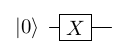
- The quantum circuit diagram for X|"0"> is as follows:
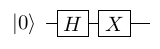
- The quantum circuit diagram for XH|"0"> is as follows:
Remember that, CNOT is the controlled NOT gate, and always operates on two qubits at once. This gate provides the quantum analogue of the classical XOR gate. The first qubit acts as a control qubit, and never changes as a result of the gate's operation. If this first qubit is |"1">, then a NOT operation is applied to the second qubit. If this first qubit is |"0">, then nothing is done to the second qubit.
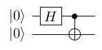
Now suppose we want to compute CNOT using |"+"> as the control qubit and |"0"> as the target qubit. Note that in the quantum circuit diagrams, we always start out with |"0">. So, we have to figure out how to get from |"0"> to |"+">. Looking at our notes from Chapter 4, Evolving Quantum States with Quantum Gates, we can see that |"+"> = H |"0">. So, we just need to apply an H gate to |"0"> before we apply CNOT. Following is the quantum circuit diagram:

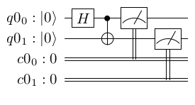
If we measure this entangled state, as we saw in the previous chapter, we will get |"00"> approximately 50% of the time and |"11"> approximately 50% of the time. Measurement can also be drawn into a quantum circuit, and our default measurement basis will be the |"0"> and |"1"> basis (also known, as we learned in Chapter 3, Quantum States, Quantum Registers, and Measurement, as the z-basis). Since measurement of a given qubit will be the |"0"> and |"1"> basis, the measurement will always produce either a |"0"> or a |"1">. We could then output the result of the measurement into a classical register, set to bit 0 if the measurement was |"0"> and to the |"1"> bit if the measurement was 1. We can represent the measurement process with the  symbol. We can represent our classical registers as starting out containing bit 0, and with double wires to distinguish them from the quantum registers. We could also choose to represent them more succinctly with a single wire with a slash through it and the label 0n (zero to the nth power), using n to indicate how many 0 bits the register should contain. This is just a shorthand, and one that you will see on IBM QX. For example, a classical register of five bits, each initialized to 0, could be visually represented by a single wire with a slash through it and the label 05. Then we can draw a double line from the symbol to the register in which we want to place the result of the measurement, thus measuring both the qubits in the circuit:
This will look as follows:

So, we know that if we prepare this circuit many times, about 50% of the time the classical registers will contain 00 after the run, and about 50% of the time the classical registers will contain 11.
Since we may want to refer to the quantum or classical registers by a name, so we can tell them apart, work with them in code, and talk about their results, we can also include a name for the register by indicating it on the left before |"0">. Here is an example of the previous circuit with labels. We label the two qubits as q0o and q01, and the two classical bits as c00 and c01:
IBM refers to its quantum circuit diagram as quantum scores. If you've ever seen music notation, a quantum score looks a bit like a musical score. In IBM QX, quantum scores can be created via the quantum composer, again a musical reference. All the gates we have learned so far are available in the quantum composer, plus a few additional gates. Although the gates we have learned so far form a universal gate set, that is, we can just use a combination of them to generate any quantum program, on a real quantum computer the fewer gates we use the better. This is because each gate takes time to execute and introduces errors.