
Injustice anywhere is a threat to justice everywhere. We are caught in an inescapable network of mutuality tied in a single garment of destiny. Whatever affects one directly affects all indirectly.
Martin Luther King Jr., Letter from a Birmingham jail, April 16,1963
In the movie, Good Will Hunting, the main character, Will Hunting, played by Matt Damon, is a janitor at a university. As he is mopping floors, he notices a problem posted on a board as a challenge to math students. The solution to the first two parts of the problem uses network analysis.
Let G be Figure 1.1 on the right.
Figure 1.1 Graph G.
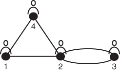
A network is a collection of points linked through some type of association. These points can represent any object or subject (e.g., people, places, and resources) and the links can represent any relationship between them (e.g., route, distance, family membership, and reporting structure). The network is graphically illustrated using lines, arcs, and symbols so the viewer can visualize and analyze the structure of the network more easily. A simple network of four points can be seen in Figure 1.1. In this network the points are people and the links are relationships between the people.
A graph is the visual representation of a set of points, frequently called vertices or nodes that are connected by line segments called edges or links. Social networks are graphs that contain a finite set or sets of actors which we call agents and the relation or relations defined between them. A social network would then be comprised of nodes representing people with the corresponding links representing the relationship between the people.
It is important to understand how to navigate through a network graph. The information gained can help us understand how information flow through a network can be used to analyze the placement of nodes within the network and gauge their significance. We will look at how to do this analysis in the next few chapters, but first we need to understand network graph navigation terminology. Figure 1.1 has four vertices or nodes. Each node is a person. Moving from one node to another along a single edge or link that joins them is a step. A walk is a series of steps from one node to another. The number of steps is the length of the walk. For instance, there is a walk of three steps from node 1 to node 3 using the steps 1 to 4, 4 to 2, and 2 to 3. A trail is a walk in which all the links are distinct, although some nodes may be included more than once. The length of a trail is the number of links it contains. For example, the length of the trail between nodes 3 and 4 is 2, where 3 to 2 is the first link, and 2 to 4 is the second link. A path is a walk in which all nodes and links are distinct. Note that every path is a trail and every trail is a walk. In application to social networks, we often focus on paths rather than trails or walks. An important property of a pair of nodes is whether or not there is a path between them. If there is a path between nodes  and
and  (say nodes 1 and node 4 in Figure 1.1), then the nodes are said to be reachable. A walk that begins and ends with the same node is called a closed walk. A cycle is a closed walk of at least three nodes. For example, the closed walk 1 to 4, 4 to 2, and 2 to 1 is a cycle as it contains three nodes and begins and ends with node 1. Cycles are important in the study of balance and clusterability in signed graphs (a topic we explore later in the book).
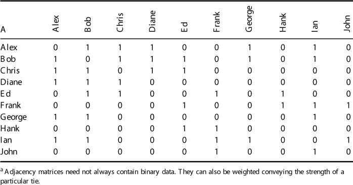
We have seen that social networks can be graphically depicted as graphs. Social networks can also be represented mathematically by matrices. For example, Figure 1.2 is a friendship graph representing friendship between a group of people. We can record how the people in the graph are related in a mathematical object known as an adjacency matrix. The adjacency matrix in this case is a square (meaning same number of rows as columns) agent by agent matrix. Table 1.1 is the adjacency matrix for Figure 1.2. Mathematically, any network can be represented by an adjacency matrix, denoted by A, which, in the simplest case, is a  symmetric matrix, where
  is the number of vertices or nodes in the network. The adjacency matrix is comprised of elements
We often represent the entire matrix with a capital letter A, B, or C. For the purpose of our friendship example, we will call the adjacency matrix A. The contents of any given cell are denoted  . For example, in the matrix above,
  , because Alex is linked to Bob. This matrix is symmetric but it does not have to be (
 is not always equal to
  ). When the matrix is symmetric, it means that relationships are reciprocated. This is called an undirected network. Symmetric matrices can be used to represent friendship, distance, conversations, and similarity in attitude, among other relationships. Directed networks are not symmetric and can be used to represent friendship that is not necessarily reciprocated, transfers of resources, and authority (such as a chain of command), among other relationships. Anything that can be represented as a graph, can also be represented as a matrix.
Figure 1.2 A social network of 10 people.
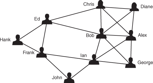
Table 1.1 Adjacency Matrix of a Friendship Graph
By convention, data is represented so that the row agent is related “to” the column agent. For example, if the relation is “trust,” then  means that agent
  trusts agent
  , but if
  then agent
 does not trust agent
  in return. The transpose of a matrix A is denoted
  . The transpose simply interchanges the rows with the columns. This will be discussed in greater detail later in the book. Table 1.2 is a table of some of the notation used to describe networks.
Table 1.2 Some Common Notations Used to Represent Networks Mathematically
| Symbol | Mathematical meaning |
 |
The sum of each value of  , as in , as in  |
 |
The adjacency matrix as in  |
 |
The transpose of the adjacency matrix as in  |
a  is sometimes denoted
  .
.
So far we have only used nodes to represent people; however, almost anything can be represented as a node or vertex. Nodes can be cities, equipment, organizations, resources, knowledge, tasks, beliefs, or any other object. A node can be anything we define it to be. Nodes that are all of the same thing (i.e. cities, equipment, organizations, etc.) are said to be of the same node class. Nodes can also exhibit attributes: a person node can have attributes such as age, gender, and the like; cities may have attributes such as population and location.
For a network to exist, the nodes must be linked by some kind of flow or relationship. Again, the link may be defined as anything that meaningfully represents the relationship. Social relations can be thought of as dyadic attributes. That is, attributes that characterize two nodes. While mainstream social science is concerned with monadic (one node) attributes (e.g., income, age, and sex), network analysis is concerned with attributes of pairs of individuals, of which binary relations are the main kind. Some examples of dyadic attributes are:
The relationship between two nodes may be either undirected or directed. Table 1.3 and Table 1.4 are the adjacency matrices for Figures 1.3a and 1.3b, respectively. An undirected relationship, Figure 1.3a, means the link is reciprocal, such as “married to,” “trades with,” or “miles between.” A directed relationship, Figure 1.3b, is where there is a movement in only one direction and this direction is indicated with an arrowhead. Examples of directed relationships are “respects,” “boss of,” and “seeks advice from.” Not all relationships are two way. For example, in Figure 1.3b, node A may seek advice from node C in a network, but node C may not seek advice from node A. The directed relationship is indicated by the arrow from node A to node C. Above each network is the adjacency matrix for that graph. You can see that there are differences between the two matrices. For example, the link between node A and node C in the undirected graph shows 1 in row A column C and 1 in row C column A, indicating that there is a link in both directions. In the directed graph, the link flows from node C to node A so the matrix shows 1 in row C column A and 0 in row A column C as the flow is only in one direction.
Table 1.3 UnDirected Matrix
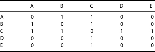
Table 1.4 Directed Matrix
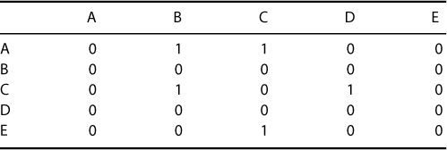
Figure 1.3 (a) Undirected and (b) directed graphs.
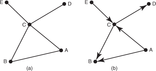
A graph will appear different depending on how the links are defined. A relationship “boss of” will result in a link with a different direction to the relationship “reports to.” Care must be taken in defining and assigning weights to relationships to ensure that accurate results are obtained for the situation under study. Unreliable input will result in unreliable output. You will notice that the diagonal cells across the matrix are each filled with a zero, indicating that there is no link between the node and itself. A link from a node to itself is termed recursive and this is not common in social network analysis. If you cut the adjacency matrix for an undirected graph along the main diagonal, one half will be a mirror image of the other half. The values of the relationships or edges for these undirected and directed graphs are binary, either 0 or 1. It is possible, however, for each relationship to be weighted or valued, carrying a larger range of values than just a binary. For example, relationships between nodes could be measured by a ranking between 0 and 5. Take the situation where you are investigating a network of employees and the people they approach for advice in carrying out their job. The link value indicates how often they confer with other colleagues for advice. A ranking of 0 could indicate they did not confer at all with that particular colleague and 5 may mean that they conferred on a daily basis.
Valued relationships can indicate amount by quantification, strength, or frequency. As the value of links change, the network can also change. Phase transitions occur when a network moves from one state to another as the weighting or value of links change. For example, as the number or value of links increases in comparison to the number of nodes, the network changes from a collection of disconnected nodes to a connected state. The network moves from one state to another.
Another way to represent network data is an edge list. An edge list is a compact way to record sparse network data (i.e., networks with few links). The edge list simply lists each link in the network beginning with the source node and ending with the target node. For example, the edge list for the directed network in Figure 1.3b is
| A | to | B |
| A | to | C |
| C | to | B |
| C | to | D |
| E | to | C |

The edge list representation is often used by computer scientists to record network data because it takes less memory than recording all of the zeros that may exist in a sparse network. This would not be particularly useful for data structures where all of the potential links had a weighted value, such as a distance network. Many social scientists find that this is an efficient method to record relational data in interviews, or observational studies as well.
Returning to the Good Will Hunting Problem, as it turns out, the adjacency matrix, A, for Figure 1.1 is the key to solving the problem. As a check on learning so far, see if you can create the adjacency matrix for Figure 1.1.
Develop the adjacency matrix for Graph G in Figure 1.1.
The next step in solving the Good Will Hunting Problem is finding the number of walks with length 3 present in the graph. Multiple compositions of the adjacency matrix,  , gives the number of walks of length
  between all nodes in the network. That is, for the adjacency matrix
  ,
,  represents the number walks of length
  from node
  to node
  . Refer to Appendix A, Matrix Algebra Primer, for a review and summary of the matrix algebra steps necessary to perform compositions of the adjacency matrix. Therefore, since

then
and
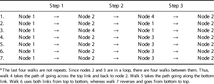
The matrix,  , reveals that there are in fact seven walks of length 3 from node 1 to node 2. Table 1.5 lists all walks of length 3 from node 1 to node 2 for this simple network. Notice from the matrix
  that there are no walks of length 3 for node 3 back to itself, and there are 12 walks of length 3 from node 2 to node 3. Thus, Will Hunting used network science in the first two steps of his four-step solution. Steps three and four use a branch of mathematics known as functional analysis and is beyond the scope of this book. A full solution can be found at the Harvard University Mathematical Archive5.
Table 1.5 3-Step Walks from Node 1 to Node 2
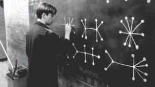
The movie Good Will Hunting proposed a second problem that relates to networks. Professor Gerald Lambeau comes to the class and announces a problem that has taken MIT professors 2 years to solve. He boldly proclaims to the class that the so-called gauntlet has been thrown down. Only strong students would dare try and solve it. The problem is, Find all homeomorphically irreducible trees of degree ten (i.e., ten vertices). In the language of network science, the problem is to find all combinations of fully connected networks with 10 nodes that contain no cycles. Essentially, it means we need to join 10 nodes together such that all nodes are connected to at least one other node. No cycles are allowed and only one link is allowed between any two nodes. Most importantly, no node can have a degree of 2. How many can you create?
Find all combinations of fully connected networks with 10 nodes that contain no cycles.
There are 10 such combinations as shown in Figure 1.4. They are listed here. How many did you find? In the movie, Will Hunting only wrote eight of them. Were you smarter than a genius?
Figure 1.4 Good Will Hunting solution.

Fun with Words
Given words: Root, Route, Brake, Break, Seen, Scene, Been, Bin, Rake, Reek. Construct a network assuming the relationship is defined by homonyms (words that sound the same). The homonyms are Root and Route, Brake and Break, Seen and Scene, and Been and Bin. The network can also be represented visually. Figure 1.5 shows a network visualization of the network consisting of the 10 words and the edge link list for the homonyms.
Figure 1.5 Edge list and network diagram for homonyms.
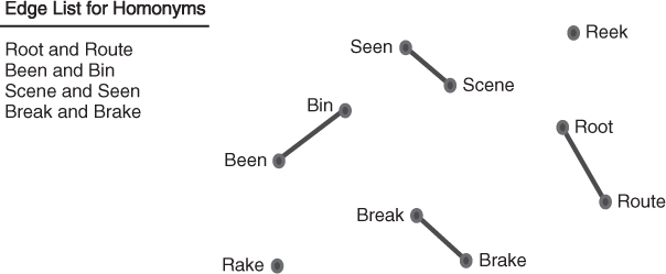
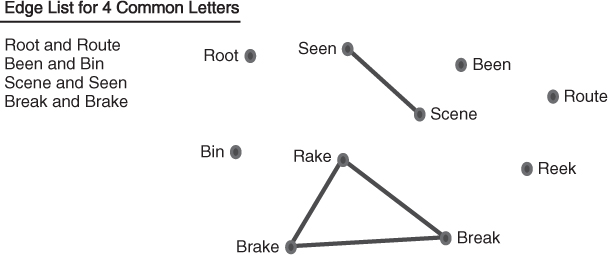
The homonym network has four edges. It is important to observe that we can also define a different relationship between the words. For example, if the relationship is defined as words that have four letters in common, a new edge list and network visualization can be created. This network also has four edges, as seen in Figure 1.6.
Figure 1.6 Edge list and network diagram for four letters in common.
Similarly, a relationship of three letters in common will produce the following edge list and network visualization, as illustrated in Figure 1.7.
Figure 1.7 Edge list and network diagram for three letters in common.
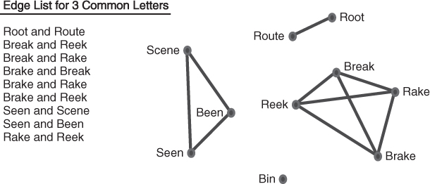
There are now 10 edges in this network. The important point here is that there is not just one relationship that can be defined on a set of nodes. The same network plotting a relationship of two letters in common will result in a much more connected network, with the edge list and visualization in Figure 1.8.
Figure 1.8 Edge list and network diagram for two letters in common.

Look at the network visualizations for two and three letters in common. The network for two letters has 20 edges, whereas the network for three letters has only 10 edges and is fragmented into smaller networks. This is another example of a phase transition. The term phase transition comes from physics and represents the point at which the network will rapidly change from fully connected to many components (or vice versa) as the threshold defining a link changes.
In social networks, friends are often different relationships than that of family, or mentorship, or even respect. A relationship can even be negative such as enemy, dislike, or contempt. The definition of what constitutes a relationship can therefore have a significant impact on the analysis of network data.
Networks of people usually relate to a structured situation or group of interest. In an organizational situation, the network of people will be employees and the relationships between them could be “reporting to,” “seeks advice from,” or any relationship defined by the viewer of that network. There is often a difference between the expected network and the actual network. Take, for example, the organizational network illustrating sources of important information between people in Figure 1.9 and Figure 1.10. This R&D organization has three main divisions led by managers Roland, Tasien, and Panks. Owing to the specialized nature of some of the work, two divisions have subsections requiring consultants; Smith manages consultants Wallis and Forge, and Tasien manages consultants Drake, Baker, and Roberts. The names in this network have been changed at the request of the organization involved. Figure 1.9 shows the formal organizational structure and Figure 1.10 illustrates the informal network structure.
Figure 1.9 R&D organization formal structure.
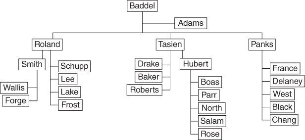
Figure 1.10 R&D Organization informal structure.

Most managers are aware of pockets of relationships that exist between their coworkers but many are not aware of the informal network structure of their entire organization or department. In Figure 1.9, Adams and North do not have prominent positions in the formal organizational network (North being fairly low rank under Hubert's management and Adams being the administrative assistant to Baddel); however, Figure 1.10 shows that both have a central role in the informal organizational structure. North, who is not ambitious, has been employed with the organization for many years and has not sought promotion. He has professional knowledge and experience that surpasses all other employees. Adams holds power due to her access to equipment and funds, and her extensive knowledge of procedures. If resources cannot be obtained through the official channels, Adams knows how to obtain them through other channels. Figure 1.10 clearly shows that the organization consists of two smaller networks, with Adams and North being the gateways between these two networks. A comparison of the formal and informal structures also indicates that very few employees go to their managers for important information. The senior managers appear to be distanced from their employees. Communications and information flows in the informal organization tend to bear little resemblance to that of the formal organization.
Military Chain of Command and Informal Power
In order to illustrate the importance of understanding social networks, here is an example of an informal network in a military organization. Consider the noncommissioned officer (NCO) support chain in an Army company. In this example organization, the first sergeant (1SG) was new to the company. This was his second assignment as a 1SG. In his previous assignment, he brought some great ideas to his company and made significant improvements. The command sergeant major (CSM) thought that the 1SG would be able to make similar improvements in our example company. Unfortunately, the 1SG's ideas were not working in the same way that it did with the previous company. Good ideas can often fail when they are implemented poorly. Understanding the informal networks will provide an insight into some important organizational dynamics.
Before we look at the informal network, we must understand the formal chain of support network in an Army company. The chain of support is illustrated in Figure 1.11.
Figure 1.11 Formal NCO chain of support.
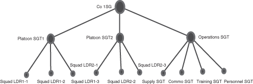
The 1SG is the senior NCO in the company. His pay grade is E-8 and he has usually served in leadership positions such as squad leader and platoon sergeant (PSG). There are two PSGs in the company as well as an operations sergeant. These NCOs are sergeants first class (SFC), or pay grade E-7. The operations sergeant is sometimes referred to as the headquarters PSG. His soldiers are responsible for providing support to the platoons. The SFCs have usually served previously as a squad leader. Their direct supervisor is typically a lieutenant. While the chain of command consists of commissioned officers, the chain of support is a parallel network of NCOs that provide the officers with advice, experience, and logistic support. Each of the platoons has three squad leaders who are staff sergeants (SSGs), pay grade E-6. The company headquarters consists of one SSG who serves as the supply sergeant and three sergeants (SGT) of pay grade E-5. The three SGTs serve as the training sergeant, the personnel sergeant, and the communications sergeant. All the nodes represented in Figure 1.11 are sized according to their rank. Thus, the 1SG is represented by a larger size node than the PSG, which is larger than the squad leader, and so on.
Does the 1SG have the power necessary to make changes in the organization? According to the formal chain of support, he does. However, in our study of this organization, the 1SG is not effective in making change. His ideas are no different than they were in a previous company where he was effective. The difference lies in the informal network of the two companies. Informal networks can be extracted in different ways.
The NCOs in this company were asked who they went to for assistance in how to do their job more effectively. The NCOs were not limited in the number of people they could list. This information represents the informal network. Individuals are not told who they have to go to for help or advice. People seek out this type of support from others for a variety of reasons. Sometimes informal relationships are determined by perceived competence, approachability, personality, common interests, or even racial/ethnic similarity. Figure 1.12 shows this informal network for our military company.
Figure 1.12 Informal NCO network.
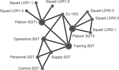
The NCOs in the first platoon, on the left, tended to follow the NCO support chain for job assistance, as did the second platoon in the middle. In the second platoon, one of the squad leaders also sought assistance from the other two squad leaders in the platoon. Perhaps this squad leader was new and looked to his peers for mentorship. Members in the headquarters platoon had a similar dynamic. The node that stands out as unusual in the informal network is the training sergeant, who consulted more than any other individual for assistance. Even the 1SG looks to the training sergeant for assistance.
There are several reasons for this informal organizational structure. The training sergeant had been serving in this capacity for almost a year and a half, which is a long time to serve in a duty position in the military. The training sergeant knew almost all of the NCOs who served in the higher battalion headquarters. He would often spend off-duty time with the battalion NCOs as well as with NCOs in his own company. In addition, he belonged to a couple of social groups that also had NCOs from different companies as members. Through this larger social network, the training sergeant was able to more effectively coordinate training resources through his friendship ties at the battalion level than other NCOs in other companies. The training sergeant was also able to mobilize his social network to find opportunities for squad leaders to send their soldiers to weapons ranges conducted by other units, use sections of training area reserved by other units, and coordinate similar training resources. The training sergeant enjoyed his position in the company. He liked the fact that senior NCOs would come to him for support. This position in the informal network gave the training sergeant power.
When the 1SG first arrived at the company, he unknowingly hurt his effectiveness in the informal network. He wanted to assert himself as a leader and decided that he needed to make sure that soldiers maintained a high standard of military appearance and bearing. The training sergeant did not make a good impression on the 1SG. The 1SG felt that the training sergeant did not maintain a professional appearance and that he was cavalier and borderline disrespectful. This may not be entirely surprising, considering the power that the training sergeant held in the informal network. The 1SG pointed out several corrections to the training sergeant and expressed his concerns about military discipline to the operations sergeant. The training sergeant was insulted and embarrassed by this first meeting. Yet, he did not openly discuss his feelings. As a result, the training sergeant was not eager to help make the new 1SG successful, nor was he enthusiastic about implementing any of the 1SGs new ideas. Further, the training sergeant disagreed with many of the 1SGs ideas. To make the company more efficient, the 1SG required NCOs to brief him on resources they were considering for their training. He would then balance those resources across the company. This of course, took away some of the power that the training sergeant enjoyed.
After a few months, it was time for the training sergeant to conduct a permanent change of station and a new NCO assumed the duties of training sergeant and the 1SGs ideas slowly made the company better. However, these improvements might have been adopted more rapidly and more effectively had the 1SG been aware of the informal social network in the company. Perhaps, if the company leadership had been able to monitor the social network, they would have prevented a relatively junior NCO from having so much power in the organization. Perhaps, the company leadership could have utilized the training sergeants informal network through appropriate incentives. In any case, this example illustrates the importance of understanding the informal social network in an organization.
Social network analysis offers more than pictures: it provides an entirely new dimension of statistical analysis for organizational behavior. Traditional analysis focuses on individual attributes. Social networks focus on relationships between individuals. Traditional analysis assumes statistical independence, whereas social network analysis focuses on dependent observations. Traditional analysis seeks to identify correlation between significant factors and a response variable. Social network analysis seeks to identify organizational structure. The underlying mathematics behind traditional analysis is calculus, the language of change. The corresponding mathematics behind social network analysis is linear algebra (Lay, 2005) and graph theory (West, 2000). These differences can be significant in terms of how someone looks at an organization.
Social network analysis provides the tools to analyze situations under study as networks, provided nodes can represent objects or individuals, and links or edges denote relationships. Network analysis has the advantage of being able to analyze entire networks such as organizations, as opposed to traditional analysis that concentrates on analyzing the significance of individual factors. In an organizational setting, network analysis enables the analyst to study the links between people, which can indicate both positive and negative relationships. By studying both the formal reporting structures as well as the informal social networks, analysts can provide valuable information to decision makers within the organization.
Here is a summary of the key points discussed in this chapter:
Go to the following URL and enter the name of a movie star to see how many links away from Kevin Bacon.
Have you heard of six degrees of separation? What does this mean? Google it!
Load the ORA software from the CASOS website (URL below). ORA is free, but you need to register, so please enter your email address.
You will find a variety of User Guides and Tutorials for download from the CASOS web site at
You will be using the LabExercise1data provided in the following table:
Using ORA: You can create a new meta-network in ORA or load previously defined meta-networks. Meta-networks comprise nodes and links. You must create a meta-network, then add node classes, and then you will be able to add links between nodes to form networks.
Double click on the ORA icon to start ORA running 
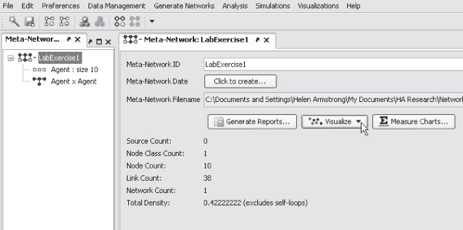
The main ORA screen will appear:

Panel 1 displays a list of the meta-networks that has been loaded into ORA, its components, and sub-networks. To view information about a particular meta-network or sub-network, single-click on the meta-network name.
Panel 2 displays information about the meta-network or sub-network highlighted in Panel 1.
Panel 3 displays information about the results of analyses run on your meta-network.
We will now create a new meta-network called LabExercise1 and enter the data in the tables for the meta-network named Lab Exercise 1 (data tables can be found in Appendix B). This meta-network has only one node class named Agent, and one network named Agent  Agent.
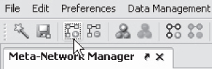
Let us begin. Start ORA by double clicking on the ORA icon. You should get the introductory screen above. Select the icon for a new meta-network.
ORA will create a meta-network in Panel 1 called New Meta-Network
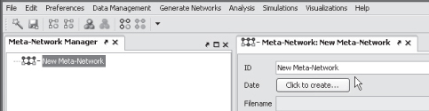
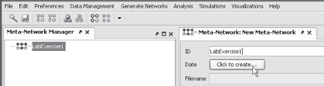
In Panel 2 enter the network ID as LabExercise1 (replacing New Meta-Network) and press Click to Create.
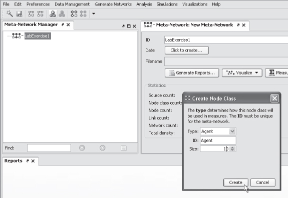
We will now add the node class Agent to the meta-network. Select the icon for a new node class.
Leave the node type and ID as Agent.
Enter 10 for the Size field in the Create Node Class dialog box to generate 10 Agent nodes. Then select Create.
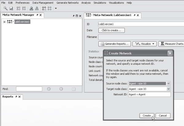
We will now create an Agent  Agent network. Select the icon for a new network.

Enter the name Agent  Agent for the relationship in the dialog box. Select Create.
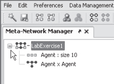
Expand the meta-network by clicking on the plus icon next to the meta-network. The plus sign will then change to minus.
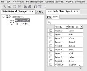
Select the Node Class Agent: size 10. Click on the Editor tab. Enter the names for the agents as follows:
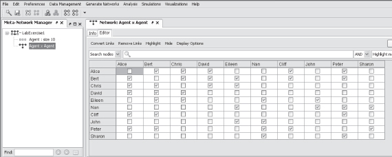
Select the network Agent  Agent; select the Editor tab in the editor window to the right; and double click on a cell to insert a tick. A tick represents 1 in the adjacency matrix for Lab Exercise 1 and no tick represents 0.
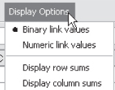
Use the Display Options tab to toggle between binary and numeric link display. What does each option do? Try them and see.
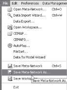
We must save our work before we go any further. Save the meta-network by selecting File  Save As. Name the meta-network LabExercise1. It will be saved as an .xml file named LabExercise1.xml.
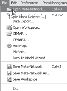
When we want to open this meta-network again, select File  Open Meta-Network
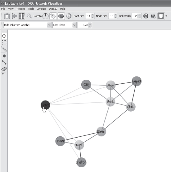
Click on the Meta-Network LabExercise1 again then choose the Visualize tab.
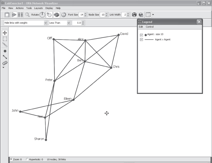
Your network visualization should look like the following:
You can toggle to change the background color between white and black by:

So that you can see the network in full, move the Legend box by clicking on the blue strip at the top and drag it.
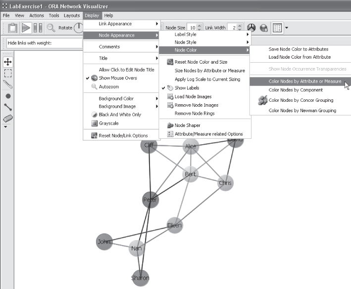
Play with  Display options
  Node Appearance and Background color to change the background to other colors, change the color and size of the nodes, etc.
By pressing the Stop/Pause layout button on the top left of the screen, you can stop the automatic formatting and reposition the nodes.

Click on a node, hold it, and drag it to where you want it positioned, then release. You will notice that the lines attached to the node will move with the node. Keep repositioning nodes until you are happy with the diagram.
Save the image to your drive by File  Save Image to File, and assign a name that relates to the exercise. Use a .jpg format for the saved image.
The arrow to the left will resume auto formatting. Well done! You have now completed Lab Exercise 1.
You have played the Kevin Bacon game; uploaded the ORA software and had it running; and opened a meta-network from file, viewed its adjacency matrix, and produced a visualization of the network.
1.1 Construct a social network of people in your class or of those known to the class.
1.2 Construct a directed graph to illustrate the following network of countries that trade together. Cameria exports to Puma and Rovia. Rovia exports to Gundi, Isicca, and Wenland. Puma exports to Klapistan. Wenland exports to Promany, Nigaly, Englore, and Isicca. Nigaly exports to Isicca and Gundi.
1.3 Construct the binary adjacency matrix for the network in Exercise 1.2.
1.4 Construct a directional network to represent the following situation. Make sure you show the direction of the relationship.
| Employee | Who they go to for advice |
| Bill | Fred, Heather, Paul |
| Fred | Mary, Paul, Julie, Heather |
| Mary | Julie |
| Gordon | Heather |
| Heather | Paul |
| Julie | Paul, Heather |
| Paul | Heather |
1.5 Construct the binary adjacency matrix for the network in Exercise 1.4.
1.6 Using an automated network analyses and visualization tool, enter the adjacency matrix for the data in the friendship graph (Fig. 1.2) and produce an image of the network using the visualization function of the tool.
1.7 Using an automated network analyses and visualization tool, complete the adjacency matrix for the informal organizational structure for the friendship graph (Fig. 1.2) and produce an image of the network using the visualization function of the tool.
Lay, D. (2005). Linear Algebra and Its Applications, 3rd updated edition. Addison Wesley.
West, D. (2000). Introduction to Graph Theory, 2nd edition. Prentice Hall.