Chapter 3: Graph Level Measures
We must all hang together, or assuredly we shall all hang separately.
Benjamin Franklin
Learning Objectives
1. Understand graph level measures of density and diameter.
2. Understand centralization measures of degree centralization, betweenness centralization, and closeness centralization.
3. Understand average centrality measures for graphs of average degree, average betweenness, average closeness, and average eigenvector.
4. Explain the difference between a graph level measure and a node/agent level measure.
5. Calculate and interpret average centralities using ORA.
Why Graph Level Measures?
Rather than focus on agents within a social network, we might be interested in some of the properties of the network as a whole. How does the organization seem to get along collectively? What is the average path length for a message to travel from one agent to the next? Do agents in this network tend to make relational connections when introduced? Can we neatly separate the network into two teams? Are there key agents who are highly central to the network while the majority of the remaining agents are not high in centrality? What does the structure of the network tell us about the ability of this network to withstand the removal of highly central agents? How does this network compare to another network of the same size and type? These are questions that could perhaps be answered given a list of agent measures, but it is much easier to look at a few graph level measures, also referred to as network level measures, to find the answers to all these questions.
3.1 Density
The density of a network is a graph or network level measure of the ratio of the number of links present given the total number of links possible. In a dense network, there are many links. In a sparse (opposite of dense) network, there are relatively few links. Before we determine how to calculate the density of a specific network, we must explore how to determine the total number of possible links that could be present in the network.
There are a couple of ways to understand how to determine the total number of possible links in a network. We have already explored this in the previous chapter when we were investigating betweenness centrality. If there are  nodes, then the number of potential combination of pairs of nodes is
  , pronounced
  choose 2. This expression can be further expressed as
  , and it describes the number of undirected or bi-directed potential links in the network. If the network is directed, then we must use a permutation instead of a combination. The potential pairs of nodes in a directed network can be expressed as
 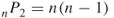 .
.
Another way to visualize the number of possible links is to consider an  adjacency matrix. To determine the total number of entries possible in a matrix, simply multiply
  , which is
  . Recall that in an adjacency matrix, the reflexive (self links) are undefined and do not exist. Therefore, we must remove
  possible entries from the
  options, which is
 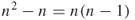 . This is equivalent to the number of permutations. If a link from node
  to node
  is the same as a link from node
  to node
  , then there are only half as many possible entries to consider. The equation becomes
  , which is equivalent to the number of combinations. The density is then the number of links present in the network, divided by the total number of possible links.
Example 3.1
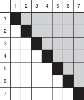
Consider a network with seven nodes. Figure 3.1 is a chart of the possible entries for links. There are seven nodes. Therefore, there exist 49 squares that could contain an entry describing a relationship. The black squares represent the reflexive links that are typically excluded. This leaves  squares. Half of the 42 squares are gray and the other 21 squares are white. If the network is undirected, then we would only consider the gray squares as these will be a mirror image of the white squares. If, however, the network is directed, then we must consider both the white and gray squares.
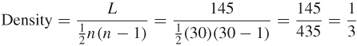
Example 3.2
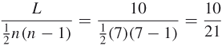
Find the density of an undirected network consisting of 30 nodes and 145 links.
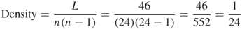
Example 3.3
Find the density of a directed network consisting of 24 nodes and 46 links.
Check on Learning
If there are 10 links in a seven-node undirected network, calculate the density.
Answer
3.2 Diameter
The diameter is a network level measure of network connectedness. The diameter describes the length of time or amount of effort needed for information to move from one end of the network to the other. The diameter is simply the longest geodesic in the network. Recall that the geodesic is the shortest path between two nodes. The shortest geodesic will, of course, be equal to 1 in the case of adjacent nodes.
Example 3.4
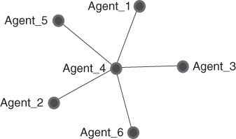
Find the diameter of the network shown in Figure 3.2.
To find the diameter, simply look for the longest geodesic. Start with a node on the periphery of the network. For example, there is a geodesic of length one starting with agent 3, {3,4}. There is a geodesic of length 2 starting with agent 3, {3,4,5}. There are no geodesics of length 3 or more. Therefore, the maximum geodesic is length 2; thus, the  .
.
Example 3.5
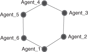
Find the diameter of the network shown in Figure 3.3.
To find the diameter, we again look for the longest geodesic. Start with a node on the periphery of the network. There is a geodesic of length 1 starting with agent 3, {3,4}. There is a geodesic of length 2 starting with agent 3, {3,4,5}. In this network, there is also a geodesic of length 3 starting with agent 3, {3,4,5,6}. There is no geodesic of length 4. The path {3,4,5,6,1} is not a geodesic because the path from agent 3 to agent 1 could also be reached through {3,2,1}, which is shorter than {3,4,5,6,1}. Thus, the  .
.
Notice the difference in the two examples. The first example (the star graph) had a diameter of 2. In this network, agent 4 quickly passed information to all the other agents in one step. No agent in the network is farther away than two steps from any other agent. In the second example (the circle graph), however, there are no brokering agents. It would take longer for an agent to pass information to the rest of the network.
Check on Learning
What is the diameter of a circle social network consisting of six agents?
Answer
The longest geodesic will be length 2, so the diameter of the network is 2.
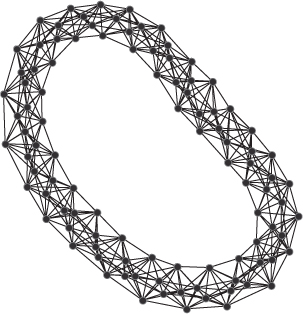
3.3 Centralization
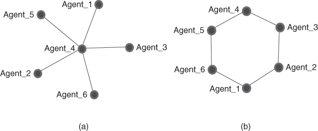
Centralization provides a network level measure of potentially exceptional nodes in the network. In other words, is there a node in the network that is much more central than typical nodes? Centralization can be calculated for any of the centrality measures. Thus, there is degree centralization, betweenness centralization, and closeness centralization. Each centralization determines the degree to which the maximum individual nodal centralities exceed the centralities of the other nodes in the network. The index will range from 0 (no node exceeds the others) to 1 (one node exceeds all others). For expository purposes, we will calculate centralization measures for the two extremes, primarily the examples from the previous sections, labeled network A (star) and network B (ring) (see Fig. 3.4). Note that the “star graph” and “circle graph” are networks that highlight the extreme boundaries of all networks, and they are bidirectional (undirectional). Directional networks will have calculated values between 0 and 1 also. The general form of centralization given by Freeman (1979) is
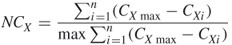
where  is the number of nodes,
  represents the individual nodal centrality values,
  is the largest value of
  for any node in the network, and
 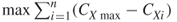 equals the maximum possible sum of differences in nodal centrality for a network of
  nodes.
3.3.1 Degree Centralization
Degree centralization reflects the relative dominance of a single node over all other nodes in the network. Networks with a high degree centralization measure are subject to fragmentation if these highly connected nodes are removed. Networks with a low degree centralization measure are less sensitive to fragmentation by the removal of nodes because no one node connects all other nodes in the networks. The degree centralization formula as expressed by Freeman (1979) is given as
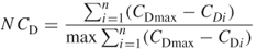
The numerator of  is calculated using the nonstandardized measure
  rather than the standardized (normalized) measure
  . The denominator is a calculation of the maximum sum of differences and is calculated by first noting that the maximum value of
  , that is,
  is
is  , which represents a network that contains one node lying adjacent to all of its neighbors. The neighbors of this one special node in turn would have only one link into the network. This is the exact representation of the star network of Figure 3.4a Network A. The structure of the graph dictates that all but one of the
  value are 1. The differences then become

Summing the differences will yield
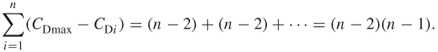
The question one might ask is whether or not this, in fact, is the maximum difference? To answer this question, we can suppose that we add a line to any pair of nodes of the star so that it becomes, say, a part of a rim of a wheel. This would make the connected nodes compared to the center yield a difference

which is smaller than  . If we remove a link, then one node will be isolate, that is, entirely unconnected. The isolate node will yield a difference of

but all the other node differences will be reduced:

Thus, 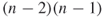 is the maximum sum of differences for degree centrality and yields
Example 3.6
Find the degree centralization of Network A.
For this network,  .
.
A centralization of 1 indicates that there is a single point of failure for the measure centrality in the network. In other words, one node is completely central, while other nodes are not central at all.
Example 3.7
Find the degree centralization of Network B.
For this network,  .
.
A centralization of 0 indicates that all the nodes have the same centrality and there is no node that is more influential than any other node.
3.3.2 Betweenness Centralization
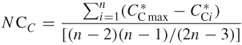
Betweenness centralization will indicate whether a sole gatekeeper exists within the network, or whether no one node controls access to all the other nodes in the network. Betweenness centralization is calculated using the standardized indices (between 0 and 1) for betweenness and is defined as
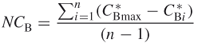
with the sum of maximum differences being equal to  .
.
Example 3.8
Find the betweenness centrality of Network A.
The betweenness centrality of Agent_4 is 1 and the betweenness centrality of all other nodes is 0. Therefore,  . Thus, the expression for betweenness centralization can be expressed as
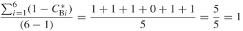
A centralization of 1 indicates that there is a single “gatekeeper” in the network. In other words, one node completely controls access to the other nodes. The other nodes do not control access to any other nodes.
Example 3.9
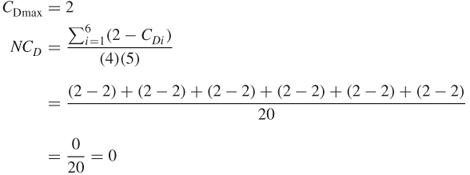
Find the betweenness centralization of Network B.
The betweenness centrality of all nodes in the network is the same and the value is 0.2. Therefore,  . Thus, the expression for betweenness centralization can be expressed as
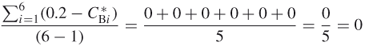
A centralization of 0 indicates that there is no single “gatekeeper” in the network. No one node controls access to the other nodes any more or less than any other node in the network.
3.3.3 Closeness Centralization
Closeness centralization will indicate the similarity of the closeness of nodes and will show whether there is a dominant node that is as close as only one step away from all other nodes in the network. Closeness centralization is calculated using the standardized indices for closeness and is defined as
with the sum of maximum differences being equal to  .
.
Example 3.10
Find the closeness centralization of Network A.
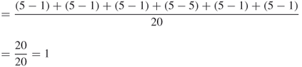
The closeness centrality of Agent_4 is 1 and the closeness centrality of all other nodes is 5/9. Therefore  . Thus, the expression for closeness centralization can be expressed as
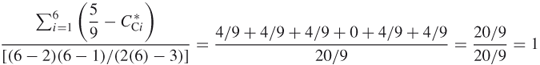
A centralization of 1 indicates that there is a single node that is one step away from every other node in the network. In other words, one node can pass information to every other node in a single step. The other nodes are at least two steps from each other.
Example 3.11
Find the closeness centralization of Network B.
The closeness centrality of all nodes in the network are the same and the value is 5/9. Therefore,  . Thus, the expression for closeness centralization can be expressed as
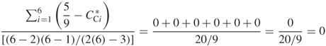
A centralization of 0 indicates that all nodes are equidistant and, therefore, require the same number of steps to traverse the network. In other words, every node passes information to every other node in the same number of steps.
3.4 Average Centralities
The averages of some centralities at a network level can provide us with valuable information when comparing different networks. We will now look at average centralities for degree, closeness, betweenness, and eigenvector and see what these average measures mean.
Average degree centrality is a measure of network density

which is a measure of the number of links present compared to the total number of links possible. Because of the way we have defined it here, this number will vary between 0 and 1 and is standardized to measure networks with varying sizes of  . Density is probably the most widely used network level measure and is regarded as a measure of group cohesion.
Average closeness centrality measures the average length of geodesics within the network.

Average betweenness centrality is the average number of agents per geodesic.

The average eigenvector centrality has a complicated mathematical expression, but it can be interpreted as follows: high average eigenvector centralities mean that, on average, agents are connected to other influential agents, that is, lower values of average eigenvector centrality indicate that there may be a small “elite group” in the network with much influence.
Check on Learning
1. What is the difference between average degree centrality and degree centralization?
Answer
1. Average degree centrality is a measure of the number of links present compared to the total number of links possible in the network. Degree centralization indicates the relative dominance of a single node over all other nodes in the network.
3.5 Network Topology
Network topology, which is the structure of the network as a whole, can tell us much about the characteristics of the network and how it might be expected to behave. Different network topologies can reflect different graph measures. The measures can be characterized by values such as their clustering coefficient, diameter, average shortest path, degree, degree distribution, and robustness. Airoldi and Carley (2005) summarizes the pure types of network topologies as follows:
- Ring lattice, where each node is connected to its neighbors.
- Small world, where each node is connected to some of its neighbors and a few distant nodes.
- Random (Erdös–Rényi), where each node is connected to a random set of the remaining nodes.
- Core-periphery, where nodes belong exclusively to either the core or the periphery, and the core and periphery nodes are connected to core nodes; however, there are no edges among periphery nodes.
- Scale free, where most of the nodes are connected to a few other nodes, while few nodes are connected to many other nodes, and formally described with a power law.
- Cellular, where nodes are divided into cells and connections are frequent between nodes within each cell, and rare between nodes in different cells.
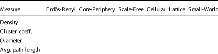
Table 3.1 lists a summary of features for each topology.
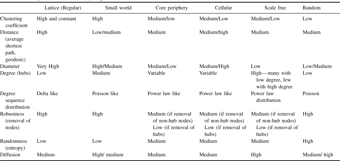
Table 3.1Comparison of Network Topologies
3.5.1 Lattice Networks
The lattice topology is a completely ordered cubic structure predominantly reflected by electrical networks, swarms of insects, schools of fish, and flocks of birds where the behavior of each individual depends on the behavior of its near neighbors.
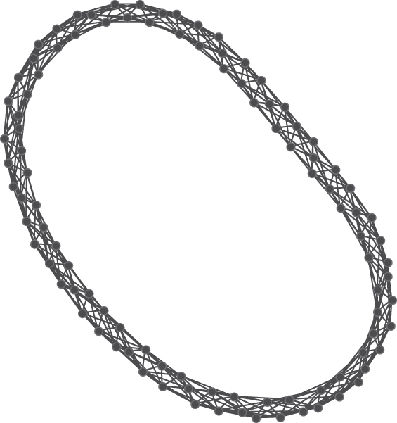
Figure 3.5 shows the structure of a network with the lattice topology comprising 100 nodes. Owing to its highly structured geometric formation, the lattice architecture is seldom realized in the real world. In real-world networks, Watts, (2003) posits that real networks more often fall between the lattice and the random structures at the two extremes of the structural spectrum. The grid or mesh structure forming the foundation of the lattice can be seen in Figure 3.6; this network has 20 nodes, each with four connections. The geometric arrangement of the nodes can be clearly seen in this diagram. Notice the absence of links that connect nodes across the graph as is usually found in small world networks. This means that information must travel around the network until it reaches its destination, making the shortest path between nodes longer than that of a small world network. Lattice networks display high clustering, low degree, and long average path lengths as there are no shortcuts. It comprises many short steps and requires many hops to reach the outer edges of the network. The short links also contribute to the higher clustering and formation of local neighborhoods. Each node in a lattice network has the same centrality measures, due to the geometrically regular structure. Each node in the network in Figure 3.6 will exhibit the same centrality measurements (scaled to between 0 and 1): 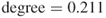 ,
,  ,
,  , and
, and  . The lattice topology is the most highly structured of topologies and the least random, situated at the opposite extreme to random (Erdös–Rényi) networks.
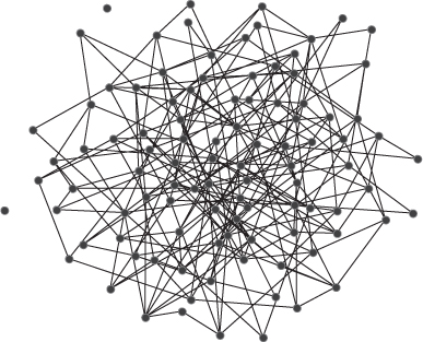
3.5.2 Small World Networks
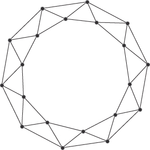
Networks with the small world topology are characterized by nodes than can reach, and can be reached by, a small number of other nodes in a small number of steps. Small world networks are sometimes referred to as six degrees of separation. There is even a web site where an individual can determine the degrees of separation of actors from Kevin Bacon (http://www.thekevinbacongame.com/. A prominent example of a small world network is the Internet, where user nodes are connected to other nodes through hyperlinks, and users can make their way through the internet network via short steps from one site to another. Figure 3.7 illustrates the structure of a small world network with 100 nodes.
In mathematical terms, the distance between two nodes chosen at random in a small world network increases in proportion to the logarithm of the number of nodes in the network. Characteristically, small world networks have small geodesics (shortest distance between nodes) and large clustering coefficients, reflecting social networks that have short distances between people and high clustering with lots of cliques. Notice the connections of nodes across the graph in Figure 3.7. These links provide greater connectivity and shortcuts for the spread of information.
The Milgram experiment by Stanley Milgram (Travers and Milgram, 1969) was the most prominent research in this area of network structure. Milgram chose 296 individuals at random from the cities of Omaha, Nebraska and Wichita, Kansas and asked them to forward a letter he provided to a target person in Boston. The individuals chosen were asked to forward the letter to the target person in Boston if they knew them directly, or, alternatively, to forward it to a person they knew who was most likely to know this target person. Of the 20% of letters that successfully reached the target person in Boston, the average length of the path was 6.5, meaning it took 6.5 steps to move between connections across the network from the original individual at the source city to the target in Boston. A later experiment by Dodds et al. (2003) used emails instead of letters, with 18 targeted individuals across 13 countries and 60,000 participants, resulting in an average path length of 4.
Substantive work has been undertaken in small world networks by Duncan Watts and Steve Strogatz (1998) and Kleinberg (2000 2001). While small world networks are high in clustering and low in distance between nodes, they also indicate a high number of hubs (see Table 3.1) that could be susceptible to attack. However, the high clustering means that alternate connections can be made easily, increasing the shortest path by only a small amount. This ensures that small world networks are robust to attack.
Latora and Marchiori (2001) confirmed in their research that neural, communication, and transport networks illustrate small world characteristics. Other examples of networks illustrating small world characteristics include the brain, the Caenorhabditis elegans worm, airline flight paths, power grids, collaboration of film actors, and signal propagation.
3.5.3 Core Periphery
Core periphery network topologies are intermediate scale (mesoscale) architectures and comprise two sets of nodes: a core set where nodes are closely tied to one another, and a peripheral set who connect more often to core members rather than other peripheral members. Research conducted by Borgatti and Everett (2000) led the way in core-periphery network structure. They added a third set of nodes possible in the core periphery structure; the nodes in the network that do not fall within the ingroup (core) and outgroup (periphery).
The core commonly displays characteristics of a cohesive subgroup with close connections and clique formations. The peripheral nodes are only sparsely connected. The core nodes are also well connected to peripheral nodes, while nodes within the core are well connected and share information and events. Those in the periphery commonly connect only with core nodes and have no interconnections at the periphery layer. Core members thus have a structural advantage over the peripheral nodes. The core periphery structure has been found in networks of the international money market, geographical systems, and economic and social networks.
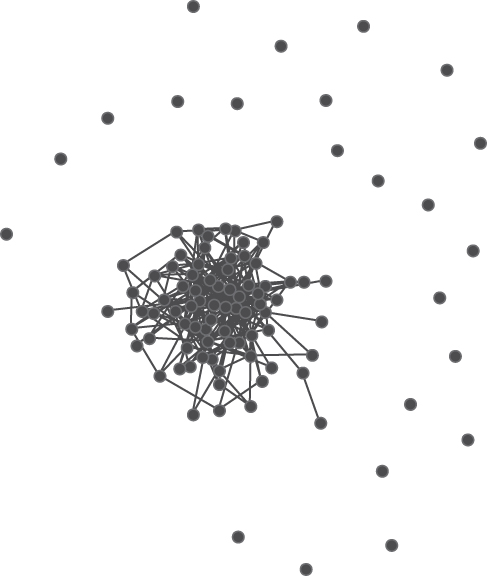
The density of core periphery networks differs between the node sets, with high density and degree in the set of core nodes, and low degree for the peripheral nodes. Figure 3.8 is a core-periphery network of 100 nodes.
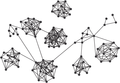
3.5.4 Cellular Networks
Substantial work has been contributed by Krebs (2002), Frantz and Carley (2005), Frantz and colleagues (2009) to cellular networks concentrating on networks of terrorists. Frantz and Carley describe cellular network structure as a collection of distributed, but sparsely connected, tightly coupled cells. These cells are often small and operate independently of one another. Researchers in terrorist networks commonly find that cells specialize in certain knowledge, resources, and tasks, and often do not know about the activities of other cells.
Krebs reported that covert networks are different from normal social networks in that terrorists minimize their connections within the network and do not forge new ties with those outside the network. The cells are tied by strong connections, often made during training; however, these ties frequently remain dormant and hidden and are only activated when needed. As such they appear to be weak ties in Granovetter's terms (Granovetter, 1973). These hidden links make the network structure difficult to discover and give it strength and resilience. The connections in covert networks take the form of trust relationships, tasks including phone calls, email, travel records, web sites, observations, and money and resources including bank account and money transfers.
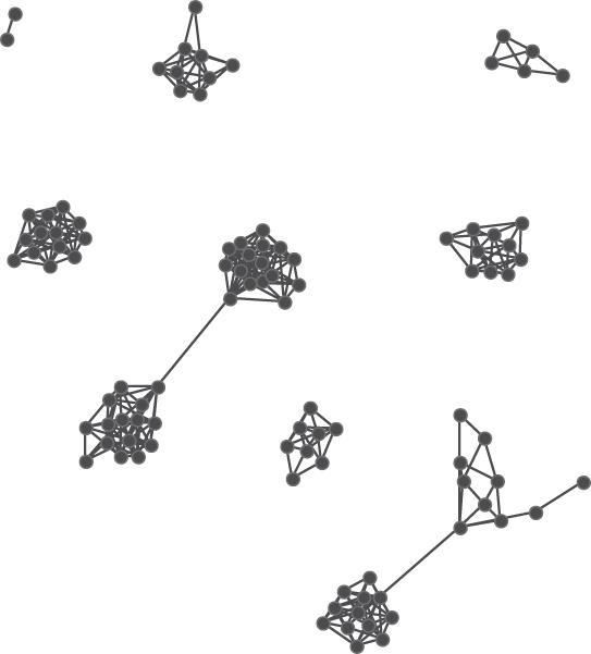
The structure of cellular network topology results in a wide network diameter owing to the low number of links between cells. While connections within the cells can be frequent, the isolation of these cells from the rest of the network affects its average shortest path and overall cohesion. If key nodes in the cells can be identified and removed, then the cell often falls into disarray owing to the lack of connections to other cells and mastermind terrorists. Carley et al. (2001) details approaches to destabilizing terrorist networks by simulating the targeting of particular nodes and evaluating the results of their removal from the network. Figure 3.9 is a cellular network of 100 nodes.
3.5.5 Scale-Free Networks
Scale-free networks are characterized by a large number of nodes with low degree and a small number of nodes with high degree (hubs). In the scale-free architecture, new nodes to the network connect to other nodes by preferential attachment, not randomly. Hence, we find that scale-free networks have clustering around hub nodes, as new nodes will prefer to link with other well-connected nodes. Some examples of scale-free networks are the world wide web, protein networks, epidemiology, and ecosystems. For example, ecosystem elements are known to form preferential connections on the basis of energy efficiency, and connections to giant hubs such as Google and Amazon on the world wide web are preferred to connecting to relatively unknown web sites. Barabási and Albert (1999) coined the actual phrase “scale-free network” as they researched the concept of preferential attachment on the world wide web and other networks with power law distributions.
Figure 3.10 illustrates the structure of a scale-free network with 100 nodes. Notice the high number of isolate nodes and those with only one or two links to other nodes. There are a few nodes toward the center of the graph that have many connections and these are the hubs to which new nodes will prefer to attach as these hubs will be more efficient, more well connected, or stronger in a key facet. Unlike small world networks, scale-free networks display a power law distribution characterized by a small number of nodes with high degree and a large number of nodes with small degree measurements. The preferential attachment of new nodes in a power law distributed network reflects the concept of the “rich get richer.” The hubs contribute substantially to the network's overall connectivity as they are the clumps of “glue” that bond the network together; however, little contribution is made by the more poorly connected nodes. Scale-free networks are more random in structure than lattice and small world networks, but less random than Erdös–Rényi (random) networks. The diameter of scale-free networks is smaller than other network architectures and this is because many nodes connect through the hubs.
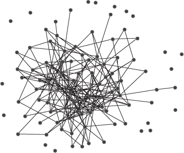
3.5.6 Random (Erdös–Rényi) Networks
Random networks are characterized by new nodes joining the network at random, without any preferential attachment as would occur in scale-free networks. This means that the linking of new nodes occurs randomly with equal probability that a new node will link to any other node, hence random networks indicate a Poisson distribution. The degree centralities of nodes in a random network are not equal as in more regular topologies such as the lattice. Owing to the irregular nature of random graphs, they rarely reflect networks in the real world, as networks grow by nodes attaching themselves to the network; and it is commonly the case that nodes have a reason for joining the network and will chose to attach on the basis of some driving force. Substantial work on random networks has been carried out by Erdös and Rényi (1960) and Watts and Strogatz (1998). Figure 3.11 illustrates the structure of random networks. The disordered nature of the network can be easily seen together with a lower clustering of nodes than that found in other topologies. Random networks have the lowest clustering coefficient of all topologies and the effect of this is the low number of hubs, or highly connected nodes. It is relatively easy to navigate to opposite sides of the network because of the formation of random links. Each node in the random network contributes approximately equally to the network's connectivity.
3.5.7 Comparison of Network Topologies
The characteristics of networks summarized in Table 3.1 compare the major types of network structures discussed in the preceding text. The columns progressively become more random from left to right (lattice, which is highly structured, to random, which has a low structure). The ratings in each cell were compiled from numerous publications on network research, too many to list individually, and the findings for each criteria were not always clear or consistent across sources.
The stability of networks is a key factor for consideration in today's uncertain global world. Of particular interest is a network's ability to diffuse information to its outer perimeters and also to withstand attack. Much of the research on diffusion relates to the adoption of innovations, which involves not only the spread of new ideas and devices but also the threshold at which the innovation is adopted. Diffusion in the context of this discussion on network topologies relates only to the spread of information and its cascading through the network to reach the peripheral nodes. While numerous studies have found that small world and scale-free structures diffuse information efficiently and quickly, research conducted by Noble, Davy, and Franks (2004) on the network structure and diffusion of innovation reported that the higher the proportion of random connections, the faster an innovative behavior spreads throughout the network. The heavily skewed distributions that result from preferential attachment appeared to slow diffusion down.
The research by Barabási et al. (2000) reported that scale-free networks are substantially more robust to the random removal of nodes than random graphs, but substantially less robust to the removal of hubs. Lewis (2009) studied the level of entropy in the different network topologies and concluded that scale free has less entropy (irregularity, chaos, or randomness) than random graphs, but more than small world or regular graphs such as the lattice. He also noted that conversely the small world graph is more structured than the random because its entropy is lower than that evident in all other classes except the regular lattice class.
However, the information in the summary table must be viewed with some caution. The results of the investigation of network topology in theoretical and simulated environments appear to differ depending on the size of the network, its density, and the way it is ordered. A number of researchers have studied the progression of graph topology from one side of the random scale to the other, gradually increasing or decreasing random node and link additions. Others take different approaches. Many researchers have found that real-world networks do not fit easily into the theoretical network topologies. Frequent findings are that real-world networks show pockets of a particular topology alongside sections showing another topology, commonly real-world networks appear to be a combination of several different network architectures. Other results (such as that of Airoldi, 2005) illustrate the difficulty in separating topological properties of cellular, core-periphery, and scale-free topologies and the concern that they share many common properties with the random topology. Airoldi's research reflects that of others and suggests that a mixture of types is a better starting point for research on real-world networks.
3.6 Summary
In this chapter, we have looked at the methods for analyzing networks at a graph level. These measures are in contrast to those we calculated at a node level. Density will tell us how well all the nodes within the network are connected. This gives us an indication of how many links there are in the network compared to how many there could be if all nodes were linked. Diameter tells us how broad the network is, or how many steps it takes to reach from one side of the network to the other. Centralization measures will tell us if there are nodes that dominate all the other nodes in degree, betweenness, and closeness centrality leading to an understanding about the network structure. Average centralities will give us information regarding the average centrality measures for all the nodes in the network. We will then be able to ascertain the average degree, betweenness, closeness, and eigenvector centrality for nodes as these provide a piece of the overall puzzle that reflects the network. We also studied the structure of different network topologies and used graph level measures to compare networks. Together with the minimum and maximum centralities for the nodes the average centralities will tell us the range of node centrality measures, thus giving us more information about the network. Together, these graph level measures and topologies will permit us to gather valuable information about the network and permit us to see similarities and differences when comparing two or more networks.
Here is a summary of the key points discussed in this chapter:
- Graph level measures tell us about the structure and nature of the entire network, whereas node level measures tell us about the centrality of each node in relation to other nodes.
- The density of a network indicates how densely the nodes are connected through the entire network when compared with total possible connections. Sparsely connected networks will not be efficient in diffusing information across the network, whereas densely connected networks will spread information much more quickly owing to the increased number of links between nodes.
- Diameter of a network measures how many steps it takes to walk across the network from one side to another. This measure will assist us in determining how long it will take for nodes on the outer edges of the network to receive information and flows when compared to nodes closer to the center of the network.
- Degree centralization will indicate if there is one node that is very high in degree centrality while the other nodes are much lower in degree centrality. This standardized measure will be 0 when all nodes have the same degree centrality and 1 when one node is connected to every other node in the network.
- Betweenness centralization indicates if there is one node that dominates in betweenness centrality while the other nodes are low in betweenness centrality. A standardized measure of 0 indicates that all nodes have the same betweenness centrality and a measure of 1 indicates that one node is between all other nodes in the network.
- Closeness centralization will tell us if one node is very high in closeness centrality while all the other nodes are low in closeness. A standardized measure of 0 will tell us that no one node is close to all other nodes and a measure of 1 indicates that one node is close to all other nodes in the network.
- Average centrality measures for nodes gives us limited information on its own; however, coupled with minimum and maximum node centrality measures, or combined with centralization measures, average centralities can provide valuable information when analyzing the structure of the network.
- Calculation of these measures via an automated tool can be achieved and Lab Exercise 3 walks the reader through this process using the ORA software provided. This can also be calculated using other automated tools.
Chapter 3 Lab Exercise
Network Level and Centralization Measures using the Organizational Risk Analyzer (ORA) Software System
Learning Objectives
1. Determine and explain average centralities for a network in ORA.
2. Determine and explain network density and diameter in ORA.
3. Determine and explain network centralization measures in ORA.
4. Learn how to generate and visualize different types of networks using ORA
1. Determine Average Centralities for Networks in ORA
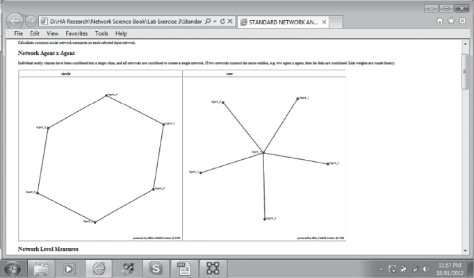
Run ORA and select the Add New Meta-network icon. Name the network “star.” Select the Add New Class Node icon and add six Agent nodes. Select the Add New Network icon and add an Agent × Agent network.
Using the image in Figure 3.4a, enter the corresponding adjacency matrix entries for this network. This is an undirected network, so all the links are reciprocated.
Save the meta-network by selecting File  Save Meta-Network As
  , then save the meta-network with the name star.xml.
Using the same steps, repeat the exercise and enter the circle network in Figure 3.4(b). Save the meta-network with the name circle.xml.
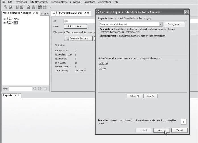
Run a Standard Network Analysis report for each network by selecting the Generate Reports tab and scrolling down to Standard Network Analysis. Select All meta-networks so that the star and circle meta-networks are ticked. Use the default parameters and produce in HTML format. (In the previous lab exercise, you generated an All Measures report. Network level measures are also shown in the All Measures report. Select Generate Report, select All Measures. Use default parameters and produce the report in HTML. Select the Analysis for network Agent × Agent link.)
Let us go back to generating the Standard Network Analysis report:
Your report for the star and circle networks should look like this:
Scroll down to see the network graphs:
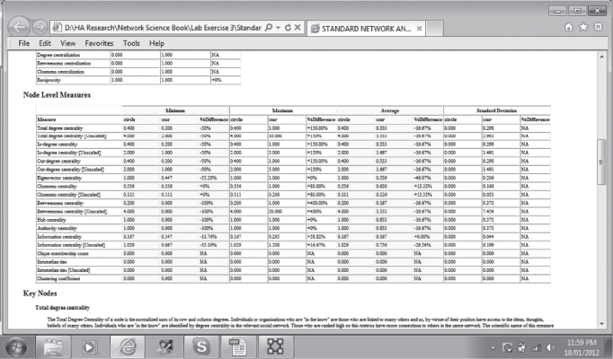
Scroll down past the Network Level measures to the Node Level Measures.
To find the average centrality measures, see column Avg in the Node Level Measures section of the Standard Network Analysis report. Note that the average centrality measures are standardized with results presented in the range 0–1.
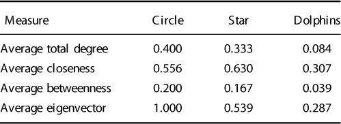
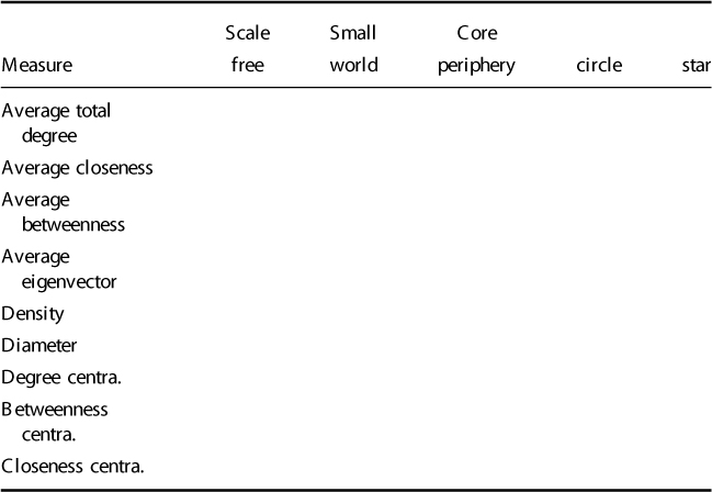
Let us compile a summary comparison table containing the average total degree, average closeness, and average betweenness:
| Measure |
Circle |
Star |
| Average total degree |
0.400 |
0.333 |
| Average closeness |
0.556 |
0.630 |
| Average betweenness |
0.200 |
0.167 |
| Average eigenvector |
1.000 |
0.539 |
Can you explain the differences in the average centralities? Here is a brief explanation:
Average total degree for the circle graph is 0.400 and is based on all nodes having the same degree centrality (each node is connected to exactly two other nodes), whereas the star graph has an average total degree of 0.333 owing to the central node that is connected to all other nodes. Both have less than half the possible links in the network.
The average closeness for the star network is 0.630 and is greater than the circle network at 0.556 as some nodes are further apart in the circle network, whereas all nodes are either one or two steps from any other node. The average betweenness for the circle network is 0.200, which is slightly greater than that for the star network at 0.167 as more nodes lie on the shortest path between two other nodes in the circle network.
The average eigenvector for the circle graph is the maximum 1.000 as all nodes are linked to other influential nodes. In the star network, the nodes are linked via Agent_4 in the center of the graph reflected by an average eigenvector value of 0.539.
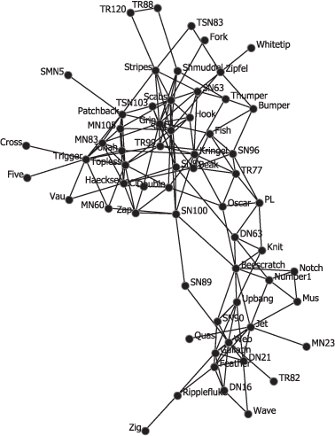
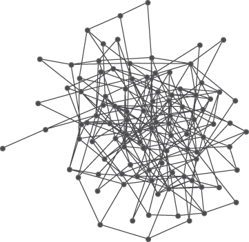
Now enter the data for the Dolphins network from Table B.6 and Table B.7 in Appendix B. Save the meta-network as dolphins.xml. You can also download this network data from the CASOS web site. This network illustrates the relationships between 62 dolphins studied in Doubtful Sound in New Zealand. The relationships plotted are individual dolphins that were seen together more often than expected by chance. For more information you can read two publications by David Lusseau that explain the research on this network of dolphins (see the references at the end of this lab exercise).
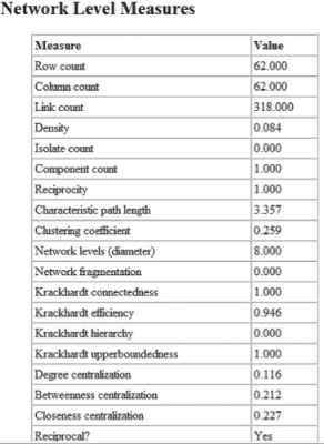
Produce a Standard Network Analysis Report for this network. Your report should look like this:
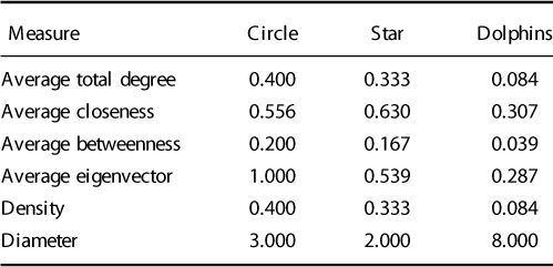
Now let us add the results for the dolphin network to our table:
We can see that the dolphin network has a lower total degree than the circle and star networks as it has a smaller proportion of possible links in the 62-node network. The size and nature of the network are also reflected in the other average centrality results, which are lower than those for the other two networks. Many dolphins have no contact whatsoever with other dolphins in the network and several key dolphins provide the connections between smaller groups within the pod. These connecting dolphins are known as boundary spanners as they are the nodes that link groups together. We will look at grouping and clustering in a future exercise.
2. Determine Network Density and Diameter
Find the network density and diameter for the three meta-networks we have loaded and add these to our table of results.
The density of the network is the same as average degree centrality at the graph level. Density measures how well nodes are connected to one another based on thedefinition of a link. A density of 0.084 means that the network is sparse, with the number of links between nodes being only a small percentage of the possible total number of links if all nodes were linked to all other nodes. This means that flow through the links will be limited to only those connections that exist, and in this case the number of links is small.
The diameter of the network describes how much effort is involved in moving from one end of the network to the other and is represented by the longest geodesic in the network. For the star graph, the maximum geodesic is length 2, thus the  . In the star network, Agent_4 is at the center of the graph and connects to all the other nodes. Agent_4 can easily and quickly pass information to the other nodes in just one step and no node in the network is more than two steps away from another node. Agent_4 is a broker in this network. For the circle graph, the diameter = 3. In this graph there is no brokering node, so it takes longer for information to travel from one node to other nodes in the network. The diameter of the dolphin network is 8. This is because it is a larger network than the circle and star and it is not as compact. Hence, it takes longer for information to travel to the outer parts of the network.
3. Determine Network Centralization measures in ORA
Using the All Measures Report and/or the Standard Network Analysis report find the centralization measures for each of the three networks and add these to our table:
Centralization measures indicate nodes that are special in that they are more central to the network than other nodes in some way. The three centralization measures—degree centralization, betweenness centralization, and closeness centralization—indicate whether an individual node has a much higher centrality than a typical node. These measures are standardized between 0 and 1. A measure of 0 indicates that no node exceeds the others (i.e., all nodes are the same) and a measure of 1 indicates one node dominates all others.
Degree centralization will indicate nodes that dominate all other nodes in the network. Removing key nodes in a network with large dominant nodes will result in division of the network into smaller groups of nodes as removal of these key nodes also removes the links, thus breaking the network apart. A measure of 1 for degree centralization indicates that one node dominates all other nodes. A measure of 0 indicates that all nodes are the same in degree centrality. Networks with low degree centralization do not have a high risk of fragmentation as there are no exceptional nodes that connect to all other nodes in the network.
Betweenness centralization indicates the presence or absence of nodes that are high in betweenness and act as gatekeepers in the network. A between centralization of 1 indicates that one node controls access to all other nodes and is most often on the shortest path between two other nodes in the network. A betweenness centralization of 0 indicates that all nodes have the same betweenness centrality.
Closeness centralization indicates whether one node is high in closeness centrality to the exclusion of others. A closeness centralization measure of 1 indicates that a central node, which is one step away from every other node in the network, exists. This central node is key to passing information to the other nodes in the network, as all other nodes are a minimum of two steps away from each other. A closeness centralization of 0 indicates that every node passes information to every other node in the same number of steps.
Looking at the results in the Standard Network Analysis report, the circle network has 0.000 for degree, betweenness, and closeness centralization. This means that all nodes have the same degree, betweenness, and closeness centralities, and no one node is more central in the network. The star network, on the other hand, has 1.000 for degree, betweenness, and closeness centralization. This means that there is one node that is totally central to the network it dominates, in degree centrality connecting to all other nodes, betweeness centrality as it lies between all other nodes as the gatekeeper in the network, and closeness centrality being only one step away from all nodes and every node being at least two steps away from every other node.
The centralization measures for the dolphin network are between those for the star and ring networks, which are the two extremes in centralization. The degree centralization is 0.116, which indicates that there are very few nodes that are high in degree centrality when compared to the other nodes in the network. Betweenness centralization is 0.212, indicating that there is no one single node that acts as a boundary spanner or gatekeeper controlling access to all other nodes in the network. Closeness centralization is 0.227, again indicating that there is little evidence of one dominant node: there is no one node that is only one step away from every other node. The nodes in this network have different closeness centrality measures as can be seen by the details in the Avg, Min/Max and Min/Max Nodes columns in the Analysis for network agent  agent section of this report. You can also see the difference in these measures for each node in the Agent-Level Measures section of this report.
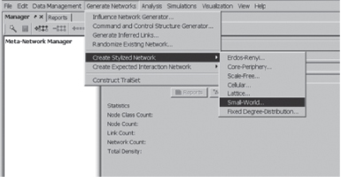
Generate Networks in ORA
The objective of this next task is to familiarize you with the generation and visualization of different types of network topologies using the ORA software. As you move through the exercise, note that the networks you generate in this lab will be slightly different than the examples in the book. The networks in this lab are generated via stochastic algorithms. It is important that you understand the characteristics of Erdös–Rènyi, core-periphery, scale-free, cellular, lattice and small-world networks.
Load ORA
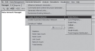
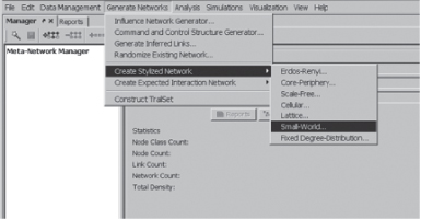
You are now going to generate some example networks. Click on the Generate Networks tab on the top left of the ORA screen, then choose Create Stylized Network. Let us start with an Erdös–Rènyi, random network.
Generate Erdös–Rènyi Network
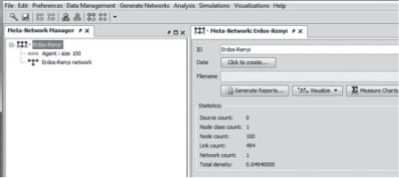
Enter the following information in the popup window. Create a new meta-network with ID: Erdös–Rènyi.
Choose the default settings as follows:
Source node class—Create the new class: is checked, type: Agent, id: Agent, size: 100.
Target node class—Create the new class is checked, type: Agent, id: Agent, size: 100.
Density should be 0.05, Allow diagonal links is unchecked, and Create a symmetric network is checked. Enter an output network ID: Erdös—Rènyi network
Press Create at the bottom of window. Then you must press Close to close this window.
Erdös will now be listed in the Meta-Network Manager section and appear as the Meta-network Erdös–Rènyi. Choose the + on the left of the meta-network name to expand the file to list the node types and networks.
Let us take a look at this network. Select the tab Visualize.
Your network will look something like this, but not exactly the same, as each randomly generated network will be slightly different! Toggle the show labels (key ring) tab to show or hide the node labels.
Now save your image, select File, then Save Image to File.
Enter File Name: Erdöos Network Example and save in JPEG format.
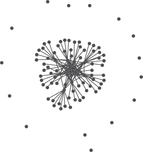
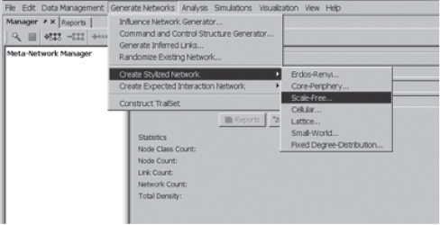
Generate Core-Periphery Network
Use the same procedure to generate the following networks using the default settings. The images will not be exactly the same, as these networks are randomly generated. Use the network type as the network ID.
Generate Networks, then Create Stylized Network, then Core Periphery. Choose the default settings.
Your Core-Periphery network should look like this:
Generate Scale-Free Network
Generate Networks, then Create Stylized Network, then Scale-Free. Choose the default settings.
Your Scale-Free network should look something like this:
Generate Cellular Network
Generate Networks, then Create Stylized Network, then Cellular. Choose the default settings.
Your Cellular network should look something like this:
Generate Lattice Network
Generate Networks, then Create Stylized Network, then Lattice. Choose the default settings.
Your Lattice network should look something like this:
Generate Small-World Network
Generate Networks, then Create Stylized Network, then Small World. Choose the default settings.
Your Small-World network should look something like this:
Build Comparative Table
Develop a table comparing the values for graph density, cluster coefficient, network diameter, average path length, and diffusion and network centralization measures. Use the following format to guide your analysis. These measures can be found by generating the All Measures report for each network in ORA. Explain your findings.
Summary
In this lab exercise, we have produced reports giving us details of average centralities, diameter and density, and network centralizations for three networks. These measures give us some tools for understanding the structure of networks and determining whether there exist any key nodes in the network. They also give us a means of comparing networks as a whole.
Load up more networks of your choice and perform the same activities. Look at the network graphs and the reports to become more familiar with these measures in different network situations.
Exercises
Generate the network graphs and adjacency matrices for five networks, all with 25 nodes, but differing topologies. All five networks are undirected. Complete the table by calculating the measures shown either manually or using an automated tool and answer the questions.
3.1 Determine the density and diameter of each network. Explain the difference between the networks.
3.2 Calculate the average degree, betweenness, closeness, and eigenvector centrality for each network. Compare these and explain the difference between the networks.
3.3 Calculate the network centralization for degree, betweenness, and closeness for each network. Compare these and explain the difference between the networks
3.4 How difficult would it be to fragment each network and how could this be done?
References
Airoldi, E. and Carley, K. (2005). Sampling algorithms for pure network topologies: a study on the stability and the separability of metric embeddings. SIGKDD Explorations Newsletter, 7(2):13–22.
Barabási, A.-L. and Albert, R. (1999). Emergence of scaling in random networks. Science, 286(5439):509–512.
Barabasi, A.-L., Albert, R., and Jeong, H. (2000). Scale-free characteristics of random networks: the topology of the world-wide web. Physica A: Statistical Mechanics and its Applications, 281(1–4):69–77.
Borgatti, S. and Everett, M. (2000). Models of core/periphery structures. Social Networks, 21(4):375–395.
Carley, K., Lee, J., and Krackhardt, D. (2001). Destabilizing terrorist networks. Connections, 3: 79–92.
Dodds, P., Muhamad, R., and Watts, D. (2003). An experimental study of search in global social networks. Science, 301(5634):827–829.
Frantz, T. and Carley, K. (2005). A formal characterization of cellular networks. CASOS Technical Report CMU-ISRI-05-109. Center for Computational Analysis of Social and Organizational Systems.
Frantz, T., Cataldo, M., and Carley, K. (2009). Robustness of centrality measures under uncertainty: Examining the role of network topology. Computational and Mathematical Organization Theory, 15(4):303–328.
Freeman, L. (1979). Centrality in social networks conceptual clarification. Social Networks, 1(3):215–239.
Granovetter, M. (1973). The strength of weak ties. American Journal of Sociology, 78(6):1360–1380.
Kleinberg, J. (2000). Navigation in a small world. Nature, 406(6798):845–845.
Kleinberg, J. (2001). Small-world phenomena and the dynamics of information. Advances in Neural Information Processing Systems (NIPS) 14.
Krebs, V. (2002). Mapping networks of terrorist cells. Connections, 24(3):43–52.
Latora, V. and Marchiori, M. (2001). Efficient behavior of small-world networks. Physical Review Letters, 87(19):198701.
Lewis, T. (2009). Network Science: Theory and Applications, 1st edition. Wiley.
Travers, J. and Milgram, S. (1969). An experimental study of the small world problem. Sociometry, 32(4):425–443.
Watts, D. (2003). Small Worlds: The Dynamics of Networks between Order and Randomness (Princeton Studies in Complexity). Princeton University Press, illustrated edition.
Watts, D. and Strogatz, S. (1998). Collective dynamics of ‘small-world’ networks. Nature, 393(6684):440–442.