As with lists, you can use the lapply and sapply functions with data frames.
Keep in mind that data frames are special cases of lists, with the list components consisting of the data frame’s columns. Thus, if you call lapply() on a data frame with a specified function f(), then f() will be called on each of the frame’s columns, with the return values placed in a list.
For instance, with our previous example, we can use lapply as follows:
> d
  kids ages
1 Jack   12
2 Jill   10
> dl <- lapply(d,sort)
> dl
$kids
[1] "Jack" "Jill"

$ages
[1] 10 12
So, dl is a list consisting of two vectors, the sorted versions of kids and ages.
Note that dl is just a list, not a data frame. We could coerce it to a data frame, like this:
as.data.frame(dl)
  kids ages
1 Jack   10
2 Jill   12
But this would make no sense, as the correspondence between names and ages has been lost. Jack, for instance, is now listed as 10 years old instead of 12. (But if we wished to sort the data frame with respect to one of the columns, preserving the correspondences, we could follow the approach presented in Extended Example: Finding the Largest Cells in a Table.)
Let’s run a logistic regression model on the abalone data we used in Section 2.9.2, predicting gender from the other eight variables: height, weight, rings, and so on, one at a time.
The logistic model is used to predict a 0- or 1-valued random variable Y from one or more explanatory variables. The function value is the probability that Y = 1, given the explanatory variables. Let’s say we have just one of the latter, X. Then the model is as follows:
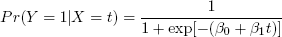
As with linear regression models, the βi values are estimated from the data, using the function glm() with the argument family=binomial.
We can use sapply() to fit eight single-predictor models—one for each of the eight variables other than gender in this data set—all in just one line of code.
1    aba <- read.csv("abalone.data",header=T)
2    abamf <- aba[aba$Gender != "I",]  # exclude infants from the analysis
3    lftn <- function(clmn) {
4       glm(abamf$Gender ˜ clmn, family=binomial)$coef
5    }
6    loall <- sapply(abamf[,-1],lftn)
In lines 1 and 2, we read in the data frame and then exclude the observations for infants. In line 6, we call sapply() on the subdata frame in which column 1, named Gender, has been excluded. In other words, this is an eight-column subframe consisting of our eight explanatory variables. Thus, lftn() is called on each column of that subframe.
Taking as input a column from the subframe, accessed via the formal argument clmn, line 4 fits a logistic model that predicts gender from that column and hence from that explanatory variable. Recall from Section 1.5 that the ordinary regression function lm() returns a class "lm" object containing many components, one of which is $coefficients, the vector of estimated βi. This component is also in the return value of glm(). Also recall that list component names can be abbreviated if there is no ambiguity. Here, we’ve shortened coefficients to coef.
In the end, line 6 returns eight pairs of estimated βi. Let’s check it out.
> loall
             Length    Diameter  Height    WholeWt    ShuckedWt  ViscWt
(Intercept)  1.275832  1.289130  1.027872  0.4300827  0.2855054  0.4829153
clmn        −1.962613 −2.533227 −5.643495 −0.2688070 −0.2941351 −1.4647507
             ShellWt    Rings
(Intercept)  0.5103942  0.64823569
col         −1.2135496 −0.04509376
Sure enough, we get a 2-by-8 matrix, with the jth column given the pair of estimated βi values obtained when we do a logistic regression using the jth explanatory variable.
We could actually get the same result using the ordinary matrix/data frame apply() function, but when I tried it, I found that method somewhat slower. The discrepancy may be due to the matrix allocation time.
Note the class of the return value of glm():
> class(loall)
[1] "glm" "lm"
This says that loall actually has two classes: "glm" and "lm". This is because the "glm" class is a subclass of "lm". We’ll discuss classes in detail in Chapter 9.
Standard Chinese, often referred to as Mandarin outside China, is officially termed putonghua or guoyu. It is spoken today by the vast majority of people in China and among many ethnic Chinese outside China, but the dialects, such as Cantonese and Shanghainese, still enjoy wide usage too. Thus, a Chinese businessman in Beijing who intends to do business in Hong Kong may find it helpful to learn some Cantonese. Similarly, many in Hong Kong may wish to improve their Mandarin. Let’s see how such a learning process might be shortened and how R can help.
The differences among the dialects are sometimes startling. The character for “down,”  , is pronounced xia in Mandarin, ha in Cantonese, and wu in Shanghainese. Indeed, because of these differences, and differences in grammar as well, many linguists consider these tongues separate languages rather than dialects. We will call them fangyan (meaning “regional speech”) here, the Chinese term.
Let’s see how R can help speakers of one fangyan learn another one. The key is that there are often patterns in the correspondences between the fangyans. For instance, the initial consonant transformation x → h seen in in the previous paragraph (xia → ha) is common, arising also in characters such as  (meaning “fragrant”), pronounced xiang in Mandarin and heung in Cantonese. Note, too, the transformation iang → eung for the non–initial consonant portions of these pronounciations, which is also common. Knowing transformations such as these could speed up the learning curve considerably for the Mandarin-speaking learner of Cantonese, which is the setting we’ll illustrate here.
We haven’t mentioned the tones yet. All the fangyan are tonal, and sometimes there are patterns there as well, potentially providing further learning aids. However, this avenue will not be pursued here. You’ll see that our code does need to make some use of the tones, but we will not attempt to analyze how tones transform from one fangyan to another. For simplicity, we also will not consider characters beginning with vowels, characters that have more than one reading, toneless characters, and other refinements.
Though the initial consonant x in Mandarin often maps to h, as seen previously, it also often maps to s, y, and other consonants. For example, the character xie,  , in the famous Mandarin term xiexie (for “thank you”) is pronounced je in Cantonese. Here, there is an x → j transformation on the consonant.
It would be very helpful for the learner to have a list of transformations and their frequencies of occurrence. This a job made for R! The function mapsound(), shown a little later in the chapter, does exactly this. It relies on some support functions, also to be presented shortly.
To explain what mapsound() does, let’s devise some terminology, illustrated by the x → h example earlier. We’ll call x the source value, with h, s, and so on being the mapped values.
Here are the formal parameters:
df: A data frame consisting of the pronunciation data of two fangyanfromcolandtocol: Names indfof the source and mapped columnssourceval: The source value to be mapped, such as x in the preceding example
Here is the head of a typical two-fangyan data frame, canman8, that would be used for df:
> head(canman8) Ch char Can Man Can cons Can sound Can tone Man cons Man sound Man tone 1yat1 yi1 y at 1 y i 1 2
ding1 ding1 d ing 1 d ing 1 3
chat1 qi1 ch at 1 q i 1 4
jeung6 zhang4 j eung 6 zh ang 4 5
seung5 shang3 s eung 5 sh ang 3 6
The function returns a list consisting of two components:
counts: A vector of integers, indexed by the mapped values, showing the counts of those values. The elements of the vector are named according to the mapped values.images: A list of character vectors. Again, the indices of the list are the mapped values, and each vector consists of all the characters that correspond to the given mapped value.
To make this concrete, let’s try it out:
> m2cx <- mapsound(canman8,"Man cons","Can cons","x")
> m2cx$counts
ch  f  g  h  j  k kw  n  s  y
15  2  1 87 12  4  2  1 81 21
We see that x maps to ch 15 times, to f 2 times, and so on. Note that we could have called sort() to m2cx$counts to view the mapped images in order, from most to least frequent.
The Mandarin-speaking learner of Cantonese can then see that if he wishes to know the Cantonese pronunciation of a word whose Mandarin romanized form begins with x, the Cantonese almost certainly begins with h or s. Little aids like this should help the learning process quite a bit.
To try to discern more patterns, the learner may wish to determine in which characters x maps to ch, for example. We know from the result of the preceding example that there are six such characters. Which ones are they? That information is stored in images. The latter, as mentioned, is a list of vectors. We are interested in the vector corresponding to ch:
> head(m2cx$images[["ch"]])
Ch char Can Man Can cons Can sound Can tone Man cons Man sound Man tone
613  chau3 xiu4 ch au 3 x iu 4
982
chau3 xiu4 ch au 3 x iu 4
982  cham4 xin2 ch am 4 x in 2
1050
cham4 xin2 ch am 4 x in 2
1050  chun3 xun2 ch un 3 x un 2
1173
chun3 xun2 ch un 3 x un 2
1173  chui4 xu2 ch ui 4 x u 2
1184
chui4 xu2 ch ui 4 x u 2
1184  chun3 xun2 ch un 3 x un 2
1566
chun3 xun2 ch un 3 x un 2
1566  che4 xie2 ch e 4 x ie 2
Now, let’s look at the code. Before viewing the code for mapsound() itself, let’s consider another routine we need for support. It is assumed here that the data frame df that is input to mapsound() is produced by merging two frames for individual fangyans. In this case, for instance, the head of the Cantonese input frame is as follows:
> head(can8) Ch char Can 1yuet3 3
naai5 6
gau2
The one for Mandarin is similar. We need to merge these two frames into canman8, seen earlier. I’ve written the code so that this operation not only combines the frames but also separates the romanization of a character into initial consonant, the remainder of the romanization, and a tone number. For example, ding1 is separated into d, ing, and 1.
We could similarly explore transformations in the other direction, from Cantonese to Mandarin, and involving the nonconsonant remainders of characters. For example, this call determines which characters have eung as the nonconsonant portion of their Cantonese pronunciation:
> c2meung <- mapsound(canman8,c("Can cons","Man cons"),"eung")We could then investigate the associated Mandarin sounds.
Here is the code to accomplish all this:
1    # merges data frames for 2 fangyans
2    merge2fy <- function(fy1,fy2) {
3       outdf <- merge(fy1,fy2)
4       # separate tone from sound, and create new columns
5       for (fy in list(fy1,fy2)) {
6          # saplout will be a matrix, init cons in row 1, remainders in row
7          # 2, and tones in row 3
8          saplout <- sapply((fy[[2]]),sepsoundtone)
9          # convert it to a data frame
10          tmpdf <- data.frame(fy[,1],t(saplout),row.names=NULL,
11             stringsAsFactors=F)
12          # add names to the columns
13          consname <- paste(names(fy)[[2]]," cons",sep="")
14          restname <- paste(names(fy)[[2]]," sound",sep="")
15          tonename <- paste(names(fy)[[2]]," tone",sep="")
16          names(tmpdf) <- c("Ch char",consname,restname,tonename)
17          # need to use merge(), not cbind(), due to possibly different
18          # ordering of fy, outdf
19          outdf <- merge(outdf,tmpdf)
20       }
21       return(outdf)
22    }
23
24    # separates romanized pronunciation pronun into initial consonant, if any,
25    # the remainder of the sound, and the tone, if any
26    sepsoundtone <- function(pronun) {
27       nchr <- nchar(pronun)
28       vowels <- c("a","e","i","o","u")
29       # how many initial consonants?
30       numcons <- 0
31       for (i in 1:nchr) {
32          ltr <- substr(pronun,i,i)
33          if (!ltr %in% vowels) numcons <- numcons + 1 else break
34       }
35       cons <- if (numcons > 0) substr(pronun,1,numcons) else NA
36       tone <- substr(pronun,nchr,nchr)
37       numtones <- tone %in% letters  # T is 1, F is 0
38       if (numtones == 1) tone <- NA
39       therest <- substr(pronun,numcons+1,nchr-numtones)
40       return(c(cons,therest,tone))
41    }
So, even the merging code is not so simple. And this code makes some simplifying assumptions, excluding some important cases. Textual analysis is never for the faint of heart!
Not surprisingly, the merging process begins with a call to merge(), in line 3. This creates a new data frame, outdf, to which we will append new columns for the separated sound components.
The real work, then, involves the separation of a romanization into its sound components. For that, there is a loop in line 5 across the two input data frames. In each iteration, the current data frame is split into sound components, with the result appended to outdf in line 19. Note the comment preceding that line regarding the unsuitability of cbind() in this situation.
The actual separation into sound components is done in line 8. Here, we take a column of romanizations, such the following:
yat1
yuet3
ding1
chat1
naai5
gau2
We split it into three columns, consisting of initial consonant, remainder of the sound, and tone. For instance, yat1 will be split into y, at, and 1.
This is a very natural candidate for some kind of “apply” function, and indeed sapply() is used in line 8. Of course, this call requires that we write a suitable function to be applied. (If we had been lucky, there would have been an existing R function that worked, but no such good fortune here.) The function we use is sepsoundtone(), starting in line 26.
The sepsoundtone() function makes heavy use of R’s substr() (for substring) function, described in detail in Chapter 11. In line 31, for example, we loop until we collect all the initial consonants, such ch. The return value, in line 40, consists of the three sound components extracted from the given romanized form, the formal parameter pronun.
Note the use of R’s built-in constant, letters, in line 37. We use this to sense whether a given character is numeric, which means it’s a tone. Some romanizations are toneless.
Line 8 will then return a 3-by-1 matrix, with one row for each of the three sound components. We wish to convert this to a data frame for merging with outdf in line 19, and we prepare for this in line 10.
Note that we call the matrix transpose function t() to put our information into columns rather than rows. This is needed because data-frame storage is by columns. Also, we include a column fy[,1], the Chinese characters themselves, to have a column in common in the call to merge() in line 19.
Now let’s turn to the code for mapsound(), which actually is simpler than the preceding merging code.
1    mapsound <- function(df,fromcol,tocol,sourceval) {
2       base <- which(df[[fromcol]] == sourceval)
3       basedf <- df[base,]
4       # determine which rows of basedf correspond to the various mapped
5       # values
6       sp <- split(basedf,basedf[[tocol]])
7       retval <- list()
8       retval$counts <- sapply(sp,nrow)
9       retval$images <- sp
10       return(retval)
11    }
Recall that the argument df is the two-fangyan data frame, output from merge2fy(). The arguments fromcol and tocol are the names of the source and mapped columns. The string sourceval is the source value to be mapped. For concreteness, consider the earlier examples in which sourceval was x.
The first task is to determine which rows in df correspond to sourceval. This is accomplished via a straightforward application of which() in line 2. This information is then used in line 3 to extract the relevant subdata frame.
In that latter frame, consider the form that basedf[[tocol]] will take in line 6. These will be the values that x maps to—that is, ch, h, and so on. The purpose of line 6 is to determine which rows of basedf contain which of these mapped values. Here, we use R’s split() function. We’ll discuss split() in detail in Section 6.2.2, but the salient point is that sp will be a list of data frames: one for ch, one for h, and so on.
This sets up line 8. Since sp will be a list of data frames—one for each mapped value—applying the nrow() function via sapply() will give us the counts of the numbers of characters for each of the mapped values, such as the number of characters in which the map x → ch occurs (15 times, as seen in the example call).
The complexity of the code here makes this a good time to comment on programming style. Some readers may point out, correctly, that lines 2 and 3 could be replaced by a one-liner:
basedf <- df[df[[fromcol]] == sourceval,]
But to me, that line, with its numerous brackets, is harder to read. My personal preference is to break down operations if they become too complex.
Similarly, the last few lines of code could be compacted to another one-liner:
list(counts=sapply(sp,nrow),images=sp)
Among other things, this dispenses with the return(), conceivably speeding up the code. Recall that in R, the last value computed by a function is automatically returned anyway, without a return() call. However, the time savings here are really small and rarely matter, and again, my personal belief is that including the return() call is clearer.