Once a mathematics PhD student whom I knew to be quite bright, but who had little programming background, sought my advice on how to write a certain function. I quickly said, “You don’t even need to tell me what the function is supposed to do. The answer is to use recursion.” Startled, he asked what recursion is. I advised him to read about the famous Towers of Hanoi problem. Sure enough, he returned the next day, reporting that he was able to solve his problem in just a few lines of code, using recursion. Obviously, recursion can be a powerful tool. Well then, what is it?
A recursive function calls itself. If you have not encountered this concept before, it may sound odd, but the idea is actually simple. In rough terms, the idea is this:
To solve a problem of type X by writing a recursive function
f():
Break the original problem of type X into one or more smaller problems of type X.
Within
f(), callf()on each of the smaller problems.Within
f(), piece together the results of (b) to solve the original problem.
A classic example is Quicksort, an algorithm used to sort a vector of numbers from smallest to largest. For instance, suppose we wish to sort the vector (5,4,12,13,3,8,88). We first compare everything to the first element, 5, to form two subvectors: one consisting of the elements less than 5 and the other consisting of the elements greater than or equal to 5. That gives us subvectors (4,3) and (12,13,8,88). We then call the function on the subvectors, returning (3,4) and (8,12,13,88). We string those together with the 5, yielding (3,4,5,8,12,13,88), as desired.
R’s vector-filtering capability and its c() function make implementation of Quicksort quite easy.
Note
This example is for the purpose of demonstrating recursion. R’s own sort function, sort(), is much faster, as it is written in C.
qs <- function(x) {
   if (length(x) <= 1) return(x)
   pivot <- x[1]
   therest <- x[-1]
   sv1 <- therest[therest < pivot]
   sv2 <- therest[therest >= pivot]
   sv1 <- qs(sv1)
   sv2 <- qs(sv2)
   return(c(sv1,pivot,sv2))
},
Note carefully the termination condition:
if (length(x) <= 1) return(x)
Without this, the function would keep calling itself repeatedly on empty vectors, executing forever. (Actually, the R interpreter would eventually refuse to go any further, but you get the idea.)
Sounds like magic? Recursion certainly is an elegant way to solve many problems. But recursion has two potential drawbacks:
It’s fairly abstract. I knew that the graduate student, as a fine mathematician, would take to recursion like a fish to water, because recursion is really just the inverse of proof by mathematical induction. But many programmers find it tough.
Recursion is very lavish in its use of memory, which may be an issue in R if applied to large problems.
Treelike data structures are common in both computer science and statistics. In R, for example, the rpart library for a recursive partioning approach to regression and classification is very popular. Trees obviously have applications in genealogy, and more generally, graphs form the basis of analysis of social networks.
However, there are real issues with tree structures in R, many of them related to the fact that R does not have pointer-style references, as discussed in Section 7.7. Indeed, for this reason and for performance purposes, a better option is often to write the core code in C with an R wrapper, as we’ll discuss in Chapter 15. Yet trees can be implemented in R itself, and if performance is not an issue, using this approach may be more convenient.
For the sake of simplicity, our example here will be a binary search tree, a classic computer science data structure that has the following property:
In each node of the tree, the value at the left link, if any, is less than or equal to that of the parent, while the value at the right link, if any, is greater than that of the parent.
Here is an example:
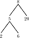
We’ve stored 8 in the root—that is, the head—of the tree. Its two child nodes contain 5 and 20, and the former itself has two child nodes, which store 2 and 6.
Note that the nature of binary search trees implies that at any node, all of the elements in the node’s left subtree are less than or equal to the value stored in this node, while the right subtree stores the elements that are larger than the value in this mode. In our example tree, where the root node contains 8, all of the values in the left subtree—5, 2 and 6—are less than 8, while 20 is greater than 8.
If implemented in C, a tree node would be represented by a C struct, similar to an R list, whose contents are the stored value, a pointer to the left child, and a pointer to the right child. But since R lacks pointer variables, what can we do?
Our solution is to go back to the basics. In the old prepointer days in FORTRAN, linked data structures were implemented in long arrays. A pointer, which in C is a memory address, was an array index instead.
Specifically, we’ll represent each node by a row in a three-column matrix. The node’s stored value will be in the third element of that row, while the first and second elements will be the left and right links. For instance, if the first element in a row is 29, it means that this node’s left link points to the node stored in row 29 of the matrix.
Remember that allocating space for a matrix in R is a time-consuming activity. In an effort to amortize the memory-allocation time, we allocate new space for a tree’s matrix several rows at a time, instead of row by row. The number of rows allocated each time will be given in the variable inc. As is common with tree traversal, we implement our algorithm with recursion.
Note
If you anticipate that the matrix will become quite large, you may wish to double its size at each allocation, rather than grow it linearly as we have here. This would further reduce the number of time-consuming disruptions.
Before discussing the code, let’s run through a quick session of tree building using its routines.
> x <- newtree(8,x)
> 3
$mat
     [,1] [,2] [,3]
[1,]   NA   NA    8
[2,]   NA   NA   NA
[3,]   NA   NA   NA

$nxt
[1] 2

$inc
[1] 3

> x <- ins(1,x,5)
> x
$mat
     [,1] [,2] [,3]
[1,]    2   NA    8
[2,]   NA   NA    5
[3,]   NA   NA   NA


$nxt
[1] 3

$inc
[1] 3

> x <- ins(1,x,6)
> x
$mat
     [,1] [,2] [,3]
[1,]    2   NA    8
[2,]   NA    3    5
[3,]   NA   NA    6

$nxt
[1] 4

$inc
[1] 3

> x <- ins(1,x,2)
> x
$mat
     [,1] [,2] [,3]
[1,]    2   NA    8
[2,]    4    3    5
[3,]   NA   NA    6
[4,]   NA   NA    2
[5,]   NA   NA   NA
[6,]   NA   NA   NA

$nxt
[1] 5

$inc
[1] 3

> x <- ins(1,x,20)
> x
$mat
     [,1] [,2] [,3]
[1,]    2    5    8
[2,]    4    3    5
[3,]   NA   NA    6
[4,]   NA   NA    2
[5,]   NA   NA   20
[6,]   NA   NA   NA

$nxt
[1] 6

$inc
[1] 3
What happened here? First, the command containing our call newtree(8,3) creates a new tree, assigned to x, storing the number 8. The argument 3 specifies that we allocate storage room three rows at a time. The result is that the matrix component of the list x is now as follows:
[,1] [,2] [,3]
[1,]   NA   NA    8
[2,]   NA   NA   NA
[3,]   NA   NA   NA
Three rows of storage are indeed allocated, and our data now consists just of the number 8. The two NA values in that first row indicate that this node of the tree currently has no children.
We then make the call ins(1,x,5) to insert a second value, 5, into the tree x. The argument 1 specifies the root. In other words, the call says, “Insert 5 in the subtree of x whose root is in row 1.” Note that we need to reassign the return value of this call back to x. Again, this is due to the lack of pointer variables in R. The matrix now looks like this:
[,1] [,2] [,3]
[1,]    2   NA    8
[2,]   NA   NA    5
[3,]   NA   NA   NA
The element 2 means that the left link out of the node containing 8 is meant to point to row 2, where our new element 5 is stored.
The session continues in this manner. Note that when our initial allotment of three rows is full, ins() allocates three new rows, for a total of six. In the end, the matrix is as follows:
[,1] [,2] [,3]
[1,]    2    5    8
[2,]    4    3    5
[3,]   NA   NA    6
[4,]   NA   NA    2
[5,]   NA   NA   20
[6,]   NA   NA   NA
This represents the tree we graphed for this example.
The code follows. Note that it includes only routines to insert new items and to traverse the tree. The code for deleting a node is somewhat more complex, but it follows a similar pattern.
1    # routines to create trees and insert items into them are included
2    # below; a deletion routine is left to the reader as an exercise
3
4    # storage is in a matrix, say m, one row per node of the tree; if row
5    # i contains (u,v,w), then node i stores the value w, and has left and
6    # right links to rows u and v; null links have the value NA
7
8    # the tree is represented as a list (mat,nxt,inc), where mat is the
9    # matrix, nxt is the next empty row to be used, and inc is the number of
10    # rows of expansion to be allocated whenever the matrix becomes full
11
12    # print sorted tree via in-order traversal
13    printtree <- function(hdidx,tr) {
14       left <- tr$mat[hdidx,1]
15       if (!is.na(left)) printtree(left,tr)
16       print(tr$mat[hdidx,3])  # print root
17       right <- tr$mat[hdidx,2]
18       if (!is.na(right)) printtree(right,tr)
19    }
20
21    # initializes a storage matrix, with initial stored value firstval
22    newtree <- function(firstval,inc) {
23       m <- matrix(rep(NA,inc*3),nrow=inc,ncol=3)
24       m[1,3] <- firstval
25       return(list(mat=m,nxt=2,inc=inc))
26    }
27
28    # inserts newval into the subtree of tr, with the subtree's root being
29    # at index hdidx; note that return value must be reassigned to tr by the
30    # caller (including ins() itself, due to recursion)
31    ins <- function(hdidx,tr,newval) {
32       # which direction will this new node go, left or right?
33       dir <- if (newval <= tr$mat[hdidx,3]) 1 else 2
34       # if null link in that direction, place the new node here, otherwise
35       # recurse
36       if (is.na(tr$mat[hdidx,dir])) {
37          newidx <- tr$nxt  # where new node goes
38          # check for room to add a new element
39          if (tr$nxt == nrow(tr$mat) + 1) {
40             tr$mat <-
41                rbind(tr$mat, matrix(rep(NA,tr$inc*3),nrow=tr$inc,ncol=3))
42          }
43          # insert new tree node
44          tr$mat[newidx,3] <- newval
45          # link to the new node
46          tr$mat[hdidx,dir] <- newidx
47          tr$nxt <- tr$nxt + 1  # ready for next insert
48          return(tr)
49       } else tr <- ins(tr$mat[hdidx,dir],tr,newval)
50    }
There is recursion in both printtree() and ins(). The former is definitely the easier of the two, so let’s look at that first. It prints out the tree, in sorted order.
Recall our description of a recursive function f() that solves a problem of category X: We have f() split the original X problem into one or more smaller X problems, call f() on them, and combine the results. In this case, our problem’s category X is to print a tree, which could be a subtree of a larger one. The role of the function on line 13 is to print the given tree, which it does by calling itself in lines 15 and 18. There, it prints first the left subtree and then the right subtree, pausing in between to print the root.
This thinking—print the left subtree, then the root, then the right subtree—forms the intuition in writing the code, but again we must make sure to have a proper termination mechanism. This mechanism is seen in the if() statements in lines 15 and 18. When we come to a null link, we do not continue to recurse.
The recursion in ins() follows the same principles but is considerably more delicate. Here, our “category X” is an insertion of a value into a subtree. We start at the root of a tree, determine whether our new value must go into the left or right subtree (line 33), and then call the function again on that subtree. Again, this is not hard in principle, but a number of details must be attended to, including the expansion of the matrix if we run out of room (lines 40–41).
One difference between the recursive code in printtree() and ins() is that the former includes two calls to itself, while the latter has only one. This implies that it may not be difficult to write the latter in a nonrecursive form.