
R contains built-in functions for your favorite math operations and, of course, for statistical distributions. This chapter provides an overview of using these functions. Given the mathematical nature of this chapter, the examples assume a slightly higher-level knowledge than those in other chapters. You should be familiar with calculus and linear algebra to get the most out of these examples.
R includes an extensive set of built-in math functions. Here is a partial list:
exp(): Exponential function, baseelog(): Natural logarithmlog10(): Logarithm base 10sqrt(): Square rootabs(): Absolute valuemin()andmax(): Minimum value and maximum value within a vectorwhich.min()andwhich.max(): Index of the minimal element and maximal element of a vectorpmin()andpmax(): Element-wise minima and maxima of several vectorssum()andprod(): Sum and product of the elements of a vectorcumsum()andcumprod(): Cumulative sum and product of the elements of a vectorround(),floor(), andceiling(): Round to the closest integer, to the closest integer below, and to the closest integer abovefactorial(): Factorial function
As our first example, we’ll work through calculating a probability using the prod() function. Suppose we have n independent events, and the ith event has the probability pi of occurring. What is the probability of exactly one of these events occurring?
Suppose first that n = 3 and our events are named A, B, and C. Then we break down the computation as follows:

P(A and not B and not C) would be pA (1 – pB) (1 – pC), and so on.
For general n, that is calculated as follows:
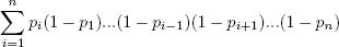
(The ith term inside the sum is the probability that event i occurs and all the others do not occur.)
Here’s code to compute this, with our probabilities picontained in the vector p:
exactlyone <- function(p) {
   notp <- 1 - p
   tot <- 0.0
   for (i in 1:length(p))
      tot <- tot + p[i] * prod(notp[-i])
   return(tot)
}
How does it work? Well, the assignment
notp <- 1 - p
creates a vector of all the “not occur” probabilities 1 – pj, using recycling. The expression notp[-i] computes the product of all the elements of notp, except the ith—exactly what we need.
As mentioned, the functions cumsum() and cumprod() return cumulative sums and products.
> x <- c(12,5,13)
> cumsum(x)
[1] 12 17 30
> cumprod(x)
[1]  12  60 780
In x, the sum of the first element is 12, the sum of the first two elements is 17, and the sum of the first three elements is 30.
The function cumprod() works the same way as cumsum(), but with the product instead of the sum.
There is quite a difference between min() and pmin(). The former simply combines all its arguments into one long vector and returns the minimum value in that vector. In contrast, if pmin() is applied to two or more vectors, it returns a vector of the pair-wise minima, hence the name pmin.
Here’s an example:
> z
     [,1] [,2]
[1,]    1    2
[2,]    5    3
[3,]    6    2
> min(z[,1],z[,2])
[1] 1
> pmin(z[,1],z[,2])
[1] 1 3 2
In the first case, min() computed the smallest value in (1,5,6,2,3,2). But the call to pmin() computed the smaller of 1 and 2, yielding 1; then the smaller of 5 and 3, which is 3; then finally the minimum of 6 and 2, giving 2. Thus, the call returned the vector (1,3,2).
You can use more than two arguments in pmin(), like this:
> pmin(z[1,],z[2,],z[3,])
[1] 1 2
The 1 in the output is the minimum of 1, 5, and 6, with a similar computation leading to the 2.
The max() and pmax() functions act analogously to min() and pmin().
Function minimization/maximization can be done via nlm() and optim().
For example, let’s find the smallest value of f(x) = x2 – sin(x).
> nlm(function(x) return(x^2-sin(x)),8)
$minimum
[1] −0.2324656

$estimate
[1] 0.4501831

$gradient
[1] 4.024558e-09

$code
[1] 1

$iterations
[1] 5
Here, the minimum value was found to be approximately −0.23, occurring at x = 0.45. A Newton-Raphson method (a technique from numerical analysis for approximating roots) is used, running five iterations in this case. The second argument specifies the initial guess, which we set to be 8. (This second argument was picked pretty arbitrarily here, but in some problems, you may need to experiment to find a value that will lead to convergence.)
R also has some calculus capabilities, including symbolic differentiation and numerical integration, as you can see in the following example.
> D(expression(exp(x^2)),"x")  # derivative
exp(x^2) * (2 * x)
> integrate(function(x) x^2,0,1)
0.3333333 with absolute error < 3.7e-15

and
You can find R packages for differential equations (odesolve), for interfacing R with the Yacas symbolic math system (ryacas), and for other calculus operations. These packages, and thousands of others, are available from the Comprehensive R Archive Network (CRAN); see Appendix B.