In the previous chapter we studied continuity of operators from a normed space X to a normed space Y. In this chapter, we will study differentiation: we will define the (Fréchet) derivative of a map f : X → Y at a point x0 ∈ X. Roughly speaking, the derivative f′(x0) of f at a point x0 will be a continuous linear transformation f′(x0) : X → Y that provides a linear approximation of f in the vicinity of x0.
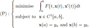
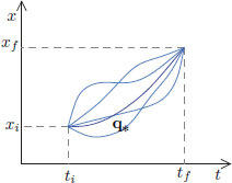
As an application of the notion of differentiation, we will indicate its use in solving optimisation problems in normed spaces, for example for real valued maps living on C1[a, b]. At the end of the chapter, we’ll apply our results to the concrete case of solving the optimisation problem
Setting the derivative of a relevant functional, arising from (P), equal to the zero linear transformation, we get a condition for an extremal curve x∗, called the Euler-Lagrange equation. Thus, instead of an algebraic equation obtained for example in the minimisation of a polynomial p : R → R using ordinary calculus, now, for the problem (P), the Euler-Lagrange equation is a differential equation. The solution of this differential equation is then the sought after function x∗ that solves the optimisation problem (P).
At the end of this chapter, we will also briefly see an application of the language developed in this chapter to Classical Mechanics, where we will describe the Lagrangian equations and the Hamiltonian equations for simple mechanical systems. This will also serve as a stepping stone to a discussion of Quantum Mechanics in the next chapter.
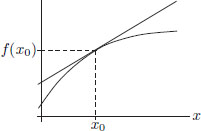
Let us first revisit the situation in ordinary calculus, where f : R → R, and let us rewrite the definition of the derivative of f at x0 ∈ R in a manner that lends itself to generalisation to the case of maps between normed spaces. Recall that for a function f : R → R, the derivative at a point x0 is the approximation of f around x0 by a straight line.
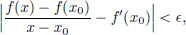
Let f : R → R and let x0 ∈ R. Then f is said to be differentiable at x0 with derivative f′(x0) ∈ R if
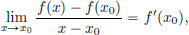
that is, for every  > 0, there exists a δ > 0 such that whenever x ∈ R satisfies 0 < |x − x0| < δ, there holds that
that is,
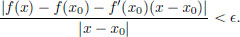
If we now imagine f instead to be a map from a normed space X to another normed space Y, then bearing in mind that the norm is a generalisation of the absolute value in R, we may try mimicking the above definition and replace the denominator |x − x0| above by ||x − x0||, and the numerator absolute value can be replaced by the norm in Y, since f(x) − f(x0) lives in Y. But what object must there be in the box below?
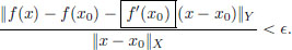
Since f(x), f(x0) live in Y, we expect the term f′(x0)(x − x0) to be also in Y. As x − x0 is in X, f′(x0) should take this into Y. So we see that it is natural that we should not expect f′(x0) to be a number (as was the case when X = Y = R), but rather it we expect it should be a certain mapping from X to Y. We will in fact want it to be a continuous linear transformation from X to Y. Why? We will see this later, but a short answer is that with this definition, we can prove analogous theorems from ordinary calculus, and we can use these theorems in applications to solve (e.g. optimisation) problems. After this rough motivation, let us now see the precise definition.
Definition 3.1. (Derivative).
Let X, Y be normed spaces, f : X → Y be a map, and x0 ∈ X.
Then f is said to be differentiable at x0 if there exists a continuous linear transformation L : X → Y such that for every > 0, there exists a δ > 0 such that whenever x ∈ X satisfies 0 < ||x − x0|| < δ, we have
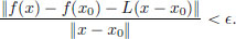
(If f is differentiable at x0, then it can be shown that there can be at most one continuous linear transformation L such that the above statement holds. We will prove this below in Theorem 3.1, page 124.)
The unique continuous linear transformation L is denoted by f′(x0), and is called the derivative of f at x0.
If f is differentiable at every point x ∈ X, then f is said to be differentiable.
Before we see some simple illustrative examples on the calculation of the derivative, let us check that this is a genuine extension of the notion of differentiability from ordinary calculus. Over there the concept of derivative was very simple, and f′(x0) was just a number. Now we will see that over there too, it was actually a continuous linear transformation, but it just so happens that any continuous linear transformation from R to R is simply given by multiplication by a fixed number. We explain this below.
Coincidence of our new definition with the old definition when we have X = Y = R, f : R → R, x0 ∈ R.
(1)Differentiable in the old sense ⇒ differentiable in the new sense.
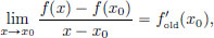
Let 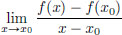 exist and be the number
Define the map L : R → R by 
Then L is a linear transformation as verified below.

(L2) For every α ∈ R and every v ∈ V,

L is continuous since |L(v)| = | (x0) · v| = |(x0)||v| for all v ∈ R. We know that
that is, for every > 0, there exists a δ > 0 such that whenever x ∈ R satisfies 0 < |x − x0| < δ, we have

that is, 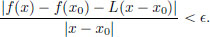
So f is differentiable in the new sense too, and  (x0) = L, that is, we have ((x0)) (v) = (x0) · v, v ∈ R.
(2)Differentiable in the new sense ⇒ differentiable in the old sense.
Suppose there is a continuous linear transformation (x0) : R → R such that for every > 0, there exists a δ > 0 such that whenever x ∈ R satisfies 0 < |x − x0| < δ, we have
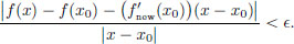
Define (x0) := (x0))(1) ∈ R. Then if x ∈ R, we have
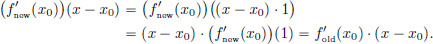
So there exists a number, namely (x0), such that for every > 0, there exists a δ > 0 such that whenever x ∈ R satisfies 0 < |x − x0| < δ,
Consequently, f is differentiable at x0 in the old sense, and furthermore, (x0) = ((x0))(1).
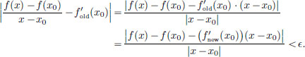
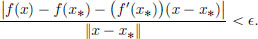
The derivative as a local linear approximation. We know that in ordinary calculus, for a function f : R → R that is differentiable at x0 ∈ R, the number f′(x0) has the interpretation of being the slope of the tangent line to the graph of the function at the point (x0, f(x0)), and the tangent line itself serves as a local linear approximation to the graph of the function. Imagine zooming into the point (x0, f′(x0)) using lenses of greater and greater magnification: then there is little difference between the graph of the function and the tangent line. We now show that also in the more general set-up when f is a map from a normed space X to a normed space Y, that is differentiable at a point x0 ∈ X, f′(x0) can be interpreted as giving a local linear approximation to the mapping f near the point x0, and we explain this below. Let > 0. Then we know that for all x close enough to x0 and distinct from x0, we have
that is, ||f(x) − f(x0) − f′(x0)(x − x0)|| < ||x − x0||. So for all x close enough to x0,

that is, f(x) − f(x0) − f′(x0)(x − x0) ≈ 0 ∈ X, and upon rearranging,

The above says that near x0, f(x) − f(x0) looks like the action of the linear transformation f′(x0) acting on x − x0. We will keep this important message in mind because it will help us calculate the derivative in concrete examples. Given an f, for which we need to find f′(x0), our starting point will always be to start with calculating f(x) − f(x0) and trying to guess what linear transformation L would give that f(x) − f(x0) ≈ L(x − x0) for x near x0. So we would start by writing f(x) − f(x0) = L(x − x0) + error, and then showing that the error term is mild enough so that the derivative definition can be verified. We will soon see this in action below, but first let us make an important remark.
Remark 3.1. In our definition of the derivative, why do we insist the derivative f′(x0) of f : X → Y at x0 ∈ X should be a continuous linear transformation—that is, why not settle just for it being a linear transformation (without demanding continuity)? The answer to this question is tied to wanting

We know this holds with the usual derivative concept in ordinary calculus when f : R → R. If we want this property to hold also in our more general setting of normed spaces, then just having f′(x0) as a linear transformation won’t do, but in addition we also need the continuity.
On the other hand, for solving optimisation problems, even if one doesn’t have differentiability at a point implying continuity at the point, one can prove useful optimisation theorems using the weaker notion of the derivative. The weaker notion is called the Gateaux derivative1, while our stronger notion is the Fréchet derivative. As we’ll only use the Fréchet derivative, we refer to our “Fréchet derivative” simply as “derivative.”
Example 3.1. Let X, Y be normed spaces, and let T : X → Y be a continuous linear transformation. We ask:

Let us do some rough work first. We would like to fill the question mark in the box below with a continuous linear transformation so that
for x close to x0. But owing to the linearity of T, we know that for all x ∈ X,

and (the right-hand side) T is already a continuous linear transformation. So we make a guess that T′(x0) = T! Let us check this now.
Let > 0. Choose any δ > 0, for example, δ = 1. Then whenever x ∈ X satisfies 0 < ||x − x0|| < δ = 1, we have

Hence T′(x0) = T. Note that as the choice of x0 was arbitrary, we have in fact obtained that for all x ∈ X, T′(x) = T! This is analogous to the observation in ordinary calculus that a linear function x  m · x has the same slope at all points, namely the number m.

Example 3.2. Consider f : C[a, b] → R,
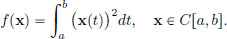
Let x0 ∈ C[a, b]. What is f′(x0)?
As before, we begin with some rough work to make a guess for f′(x0) and we seek a continuous linear transformation L so that for x ∈ C[a, b] near x0, f(x) − f(x0) ≈ L(x − x0). We have
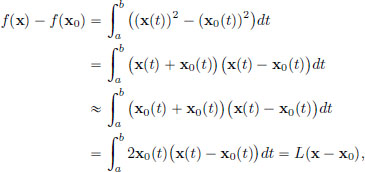
where L : C[a, b] → R is given by
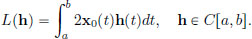
This L is a continuous linear transformation, since it is a special case of Example 2.11, page 72 (when A := 2·x0 and B = 0). Let us now check that the “-δ definition of differentiability” holds with this L. For x ∈ C[a, b],
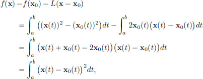
and so
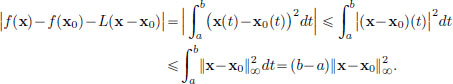
So if 0 < ||x − x0||∞, then
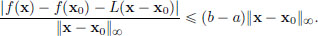
Let > 0. Set δ := /(b − a). Then δ > 0 and if 0 < ||x − x||∞ < δ,

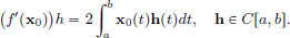
So f′(x0) = L. In other words, f′(x0) is the continuous linear transformation from C[a, b] to R given by
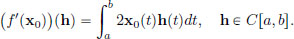
So as opposed to the ordinary calculus case, one must stop thinking of the derivative as being a mere number, but instead, in the context of maps between normed spaces, the derivative at a point is itself a map, in fact a continuous linear transformation. So the answer to the question
should always begin with the phrase
“f′(x0) is the continuous linear transformation from X to Y given by ···”.
To emphasise this, let us see some particular cases of our calculation of f′(x0) above, for specific choices of x0.
In particular, we have that the derivative of f at the zero function 0, namely f′(0), is the zero linear transformation 0 : C[a, b] → R that sends every h ∈ C[a, b] to the number 0: 0(h) = 0, h ∈ C[a, b].
Similarly, 
Exercise 3.1. Consider f : C[0, 1] → R given by 
Let x0 ∈ C[0, 1]. What is f′(x0)? What is f′(0)?
We now prove that something we had mentioned earlier, but which we haven’t proved yet: if f is differentiable at x0, then its derivative is unique.
Theorem 3.1. Let X, Y be normed spaces. If f : X → Y is differentiable at x0 ∈ X, then there is a unique continuous linear transformation L such that for every > 0, there is a δ > 0 such that whenever x ∈ X satisfies 0 < ||x − x0|| < δ, there holds
Proof. Suppose that L1, L2 : X → Y are two continuous linear transformations such that for every > 0, there is a δ > 0 such that whenever x ∈ X satisfies 0 < ||x − x0|| δ, there holds
Suppose that L1(h0) ≠ L2(h0) for some h0 ∈ X. Clearly h0 ≠ 0 (for otherwise L1(0) = 0 = L2(0)!). Take = 1/n for some n ∈ N. Then there exists a δn > 0 such that whenever x ∈ X satisfies 0 < ||x − x0|| < δn, the inequalities (3.1), (3.2) hold.
with  we have that x ≠ x0, and
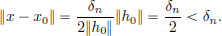
So (3.1), (3.2) hold for this x. The triangle inequality gives

Upon rearranging, we obtain 
As the choice of n ∈ N was arbitrary, it follows that ||L1(h0) − L2(h0)|| = 0, and so L1(h0) = L2(h0), a contradiction. This completes the proof.

Exercise 3.2. (Differentiability ⇒ continuity).
Let X, Y be normed spaces, x0 ∈ X, and f : X → Y be differentiable at x0.
Prove that f is continuous at x0.
Exercise 3.3. Consider f : C1[0, 1] → R defined by f(x) = (x′(1))2, x ∈ C1[0, 1]. Is f differentiable? If so, compute f′(x0) at x0 ∈ C1[0, 1].
Exercise 3.4. (Chain rule).
Given distinct x1, x2 in a normed space X, define the straight line γ : R → X passing through x1, x2 by γ(t) = (1 − t)x1 + tx2, t ∈ R.
(1)Prove that if f : X → R is differentiable at γ(t0), for some t0 ∈ R, then f  γ : R → R is differentiable at t0 and (fγ)′(t0)) = f′(γ(t0))(x2 − x1).
(2)Deduce that if g : X → R is differentiable and g′(x) = 0 at every x ∈ X, then g is constant.
From ordinary calculus, we know the following two facts that enable one to solve optimisation problems for f : R → R.
Fact 1. If x∗ ∈ R is a minimiser of f, then f′(x∗) = 0.
Fact 2. If f″(x)  0 for all x ∈ R and f′(x∗) = 0, then x∗ is a minimiser of f.
The first fact gives a necessary condition for minimisation (and allows one to narrow the possibilities for minimisers — together with the knowledge of the existence of a minimiser, this is a very useful result since it then tells us that the minimiser x∗ has to be one which satisfies f′(x∗) = 0). On the other hand, the second fact gives a sufficient condition for minimisation.
Analogously, we will prove the following two results in this section, but now for a real-valued function f : X → R on a normed space X.
Fact 1. If x∗ ∈ X is a minimiser of f, then f′(x∗) = 0.
Fact 2. If f is convex and f′(x∗) = 0, then x∗ is a minimiser of f.
We mention that there is no loss of generality in assuming that we have a minimisation problem, as opposed to a maximisation one. This is because we can just look at −f instead of f. (If f : S → R is a given function on a set S, then defining −f : S → R by (−f)(x) = −f(x), x ∈ S, we see that x∗ ∈ S is a maximiser for f if and only if x∗ is a minimiser for −f .)
Optimisation: necessity of vanishing derivative
Theorem 3.2. Let X be a normed space, and let f : X → R be a function that is differentiable at x∗ ∈ X . If f has a minimum at x∗, then f′(x∗) = 0.
Let us first clarify what 0 above means: 0 : X → R is the continuous linear transformation that sends everything in X to 0 ∈ R: 0(h) = 0, h ∈ X.
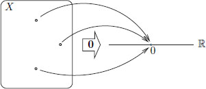
So to say that “f′(x∗) = 0” is the same as saying that for all h ∈ X, (f′(x∗))(h) = 0.
Proof. Suppose that f′(x∗) ≠ 0. Then there exists a vector h0 ∈ X such that (f′(x∗))(h0) ≠ 0. Clearly this h0 must be a nonzero vector (because the linear transformation f′(x0) takes the zero vector in X to the zero vector in R, which is 0). Let > 0. Then there exists a δ > 0 such that whenever x ∈ X satisfies 0 < ||x − x∗|| < δ, we have
Thus whenever 0 < ||x − x∗|| < δ, we have
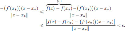
Hence whenever 0 < ||x − x∗|| < δ, 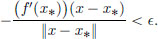
Now we will construct a special x using the h0 from before. Take
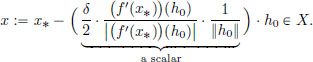
Then x ≠ x∗ and 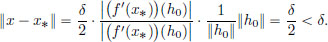
Using the linearity of f′(x0), we obtain
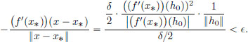
Thus, |(f′(x∗))(h0)| < ||h0||. As > 0 was arbitrary, |(f′(x∗))(h0)| = 0, and so (f′(x∗))(h0) = 0, a contradiction.
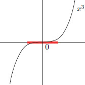
We remark that the condition f′(x∗) = 0 is a necessary condition for x∗ to be a minimiser, but it is not sufficient. This is analogous to the situation to optimisation in R: if we look at f : R → R given by f(x) = x3, x ∈ R, then with x∗ := 0, we have that f′(x∗) = 3x∗2 = 3 · 02 = 0, but clearly x∗ = 0 is not a minimiser of f.
Example 3.3. Let f : C[0, 1] → R be given by f(x) = (x(1))3, x ∈ C[0, 1]. Then f′(0) = 0. (Here the 0 on the left-hand side is the zero function in C[0, 1], while the 0 on the right-hand side is the zero linear transformation 0 : C[0, 1] → R.) Indeed, given > 0, we may set δ := min{, 1}, and then we have that whenever x ∈ C[0, 1] satisfies 0 < ||x − 0||∞ < δ,

But 0 is not a minimiser for f. For example, with x := −α · 1 ∈ C[0, 1], where α > 0, we have f(x) = (−α)3 = −α3 < 0 = f(0), showing that 0 is not2 a minimiser.
Exercise 3.5. Let f : C [a, b] → R be given by 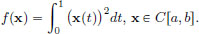
In Example 3.2, page 122, we showed that if x0 ∈ C [a, b], then f′(x0) is given by
(1)Find all x0 ∈ C[a, b] for which f′(x0) = 0.
(2)If we know that x∗ ∈ C[a, b] is a minimiser for f, what can we say about x∗?
Optimisation: sufficiency in the convex case
We will now show that if f : X → R is a convex function, then a vanishing derivative at some point is enough to conclude that the function has a minimum at that point. Thus the condition “f″(x) 0 for all x ∈ R” from ordinary calculus when X = R, is now replaced by “f is convex” when X is a general normed space. We will see that in the special case when X = R (and when f is twice continuously differentiable), convexity is precisely characterised by the second derivative condition above. We begin by giving the definition of a convex function.
Definition 3.2. (Convex set, convex function) Let X be a normed space.
(1)A subset C ⊂ X is said to be a convex set if for every x1, x2 ∈ C, and all α ∈ (0, 1), (1 − α) · x1 + α · x2 ∈ C.
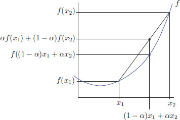
(2)Let C be a convex subset of X. A map f : C → R is said to be a convex function if for every x1, x2 ∈ C, and all α (0, 1),

The geometric interpretation of the inequality (3.3), when X = R, is shown below: the graph of a convex function lies above all possible chords.
Exercise 3.6. Let a < b, ya, yb be fixed real numbers.
Show that S := {x ∈ C1[a, b] : x(a) = ya and x(b) = yb} is a convex set.
Exercise 3.7. (||·||) is a convex function).
If X is a normed space, then prove that the norm x ||x|| : X → R is convex.
Exercise 3.8. (Convex set versus convex function).
Let X be a normed space, C be a convex subset of X, and let f : C → R. Define the epigraph of f by 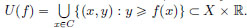
Intuitively, we think of U(f) as the “region above the graph of f ”. Show that f is a convex function if and only if U(f) is a convex set.
Exercise 3.9. Suppose that f : X → R is a convex function on a normed space X.
If n ∈ N, x1, ···, xn ∈ X, then 
Convexity of functions living in R.
We will now see that for twice differentiable functions f : (a, b) → R, convexity of f is equivalent to the condition that f″(x) 0 for all x ∈ (a, b). This test will actually help us to show convexity of some functions on spaces like C1[a, b].
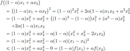
If one were to use the definition of convexity alone, then the verification can be cumbersome. Consider for example the function f : R → R given by f(x) = x2, x ∈ R. To verify that this function is convex, we note that for x1, x2 ∈ R and α ∈ (0, 1),
On the other hand, we will now prove the following result.
Theorem 3.3. Let f : (a, b) → R be twice continuously differentiable. Then f is convex if and only if for all x ∈ (a, b), f″(x) 0.
The convexity of x x2 is now immediate, as 
Example 3.4. We have 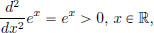 and so x ex is convex. Consequently, for all x1, x2 ∈ R and all α ∈ (0, 1), we have the inequality e(1−α)x1 +αx2
  (1 − α)ex1 + αex2 .
Exercise 3.10. Consider the function f : R → R given by  Show that f is convex.
Proof. (Of Theorem 3.3.) Only if part: Let x, y ∈ (a, b) and x < u < y.
Set  Then α ∈ (0, 1), and
  As f is convex,

that is,

From (3.4), (y − x) f(u) (u − x) f(y) + (y − x + x −y) f(x), that is,

and so

From (3.4), we also have (y − x)f(u) (u − y + y − x)f(y) + (y − u)f(x), that is, (y − x)f(u) − (y − x)f(y) (u − y)f(y) − (u − y)f(x), and so
Combining (3.5) and (3.6), 
Passing the limit as u  x and u
  y,
y, 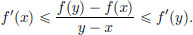
Hence f′ is increasing, and so 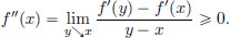
Consequently, for all x ∈ R, f″(x) 0.
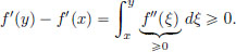
If part: Since f″(x) 0 for all x ∈ (a, b), it follows that f′ is increasing. Indeed by the Fundamental Theorem of Calculus, if a < x < y < b, then
Now let a < x < y < b, α ∈ (0, 1), and u := (1 − α)x + αy. Then x < u < y.
By the Mean Value Theorem, 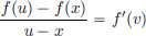 for some v ∈ (x, u).
Similarly,  for some w ∈ (u, y).
As w > v, we have f′(w) f′(v), and so

Rearranging, we obtain

Thus f is convex.
Example 3.5. Consider the function f : C[a, b] → R given by
Is f convex? We will show below that f is convex, using the convexity of the map ξ ξ2 : R → R. Let x1, x2 ∈ C[a, b] and α ∈ (0, 1). Then for all a, b ∈ R, ((1 − α)a + αb)2 (1 − α)a2 + αb2. Hence for each t ∈ [a, b], with a := x1(t), b := x2(t), we obtain

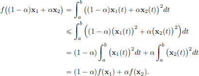
Consequently, f is convex.
Exercise 3.11. (Convexity of the arc length functional.)
Let f : C1[0, 1] → R, be given by 
Prove that f is convex.
Example 3.6. Let us revisit Example 0.1, page viii.
There S := {x ∈ C1[0, T] : x(0) = 0 and x(T) = Q}, and f : S → R was given by
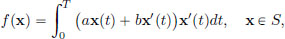
where a, b, Q > 0 are constants. Let us check that f is convex. The convexity of the map
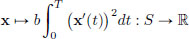
follows from the convexity of η η2 : R → R. The map
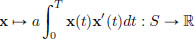
is constant on S because

and so this map is trivially convex. Hence f, being the sum of two convex functions, is convex too.
We now prove the following result on the sufficiency of the vanishing derivative for a minimiser in the case of convex functions.
Theorem 3.4.
Let X be a normed space and f : X → R be convex and differentiable. If x∗ ∈ X is such that f′(x∗) = 0, then f has a minimum at x∗ .
Proof. Suppose that x0 ∈ X and f(x0) < f(x∗). Define φ : R → R by φ(t) = f(tx0 + (1 − t)x∗), t ∈ R. The function φ is convex, since if α ∈ (0, 1) and t1, t2 ∈ R, then we have
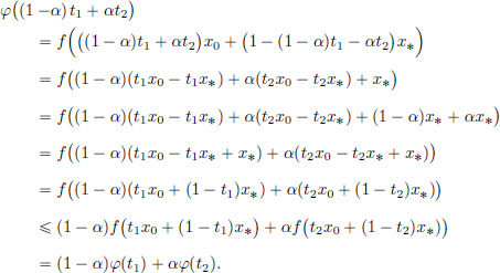
Also, from Exercise 3.4 on page 125, φ is differentiable at 0, and

We have φ(1) = f(x0) < f(x∗) = φ(0). By the Mean Value Theorem, there exists a θ ∈ (0, 1) such that
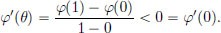
But this is a contradiction because φ is convex (and so φ′ must be increasing; see the proof of the “only if” part of Theorem 3.3).
Thus there cannot exist an x0 ∈ X such that f(x0) < f(x∗).
Consequently, f has a minimum at x∗.
Exercise 3.12. Consider 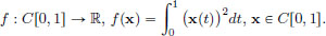
Let x0 ∈ C[0, 1]. From Example 3.2, page 122, f′(x0) : C[0, 1] → R is given by

Prove that f′(x0) = 0 if and only if x0(t) = 0 for all t ∈ [0, 1].
We have also seen that in Example 3.5, page 131, that f is a convex function.
Find all solutions to the optimisation problem 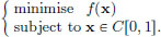
Theorem 3.5. Let
(1)x∗ ∈ S = {x ∈ C1[a, b] : x(a) = ya, x(b) = yb},
(2)
(3)
(4)X := {h ∈ C1[a, b] : h(a) = 0, x(bh = 0},
(5) : X → R be given by (h) = f(x∗ +
  ), h ∈ X .
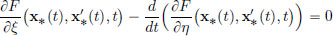
Then ′(0) = 0 if and only if x∗ ∈ S satisfies the Euler-Lagrange equation:

Definition 3.3. Such an x∗ ∈ S, which satisfies the Euler-Lagrange equation, is said to be stationary for the functional f.
Note that X defined above in Theorem 3.5 is a vector space, since it is a subspace of C1[0, 1] (Exercise 1.3, page 7), and it inherits the ||·||1,∞-norm from C1[0, 1]. To prove Theorem 3.5, we will need the following result.
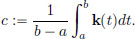
Lemma 3.1. (“Fundamental lemma of the calculus of variations”). If k ∈ C[a, b] is such that

then there exists a constant c such that k(t) = c for all t ∈ [a, b].
Of course, if k ≡ c, then by the Fundamental Theorem of Calculus,

for all h ∈ C1[a, b] that satisfy h(a) = h(b) = 0. The remarkable thing is that the converse is true, namely that the special property in the box forces k to be a constant.
(If k ≡ c, then
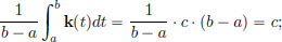
so the c defined above is the constant that k “is supposed to be”.)
Define h0 : [a, b] → R by 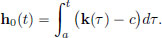
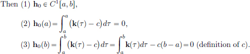
Thus 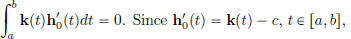 Since h′0(t) = k(t) − c, t ∈ [a, b], we obtain
Thus k(t) − c = 0 for all t ∈ [a, b], and so k ≡ c.
Proof. (Of Theorem 3.5). We note that h ∈ X if and only if x∗ + h ∈ S.

and so x∗ + h ∈ S.
Vice versa, if x∗ + h ∈ S, then

Consequently, h ∈ X .) Thus is well-defined.
What is ′(0)? For h ∈ X, we have
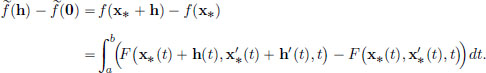
By Taylor’s Formula for F, we know that
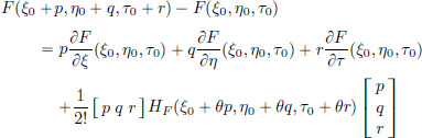
for some θ such that 0 < θ < 1. We will apply this for each fixed t ∈ [a, b], with ξ0 := x∗(t), p := h(t), η0 := x′∗(t), q := h′(t), τ0 := t, r := 0, and we will obtain a θ ∈ (0, 1) for which the above formula works. If I change the t, then I will get a possibly different θ ∈ (0, 1). So we have that the θ depends on t ∈ [a, b]. This gives rise to a function Θ : [a, b] → (0, 1) so that
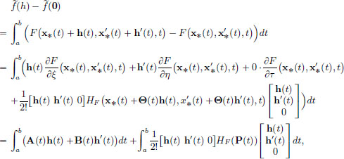
where
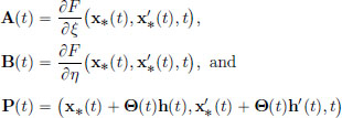
and HF (·) denotes the Hessian of F:
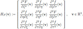
From the above, we make a guess for ′(0): define L : X → R by
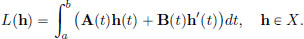
We have seen that L is a continuous linear transformation in Example 2.11, page 72. For h ∈ X,
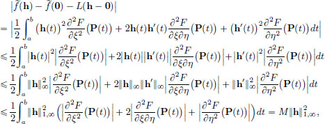
where

We note that for each t ∈ [a, b], the point

in R3 belongs to a ball with centre (x∗(t), x′∗(t), t) and radius ||h||1,∞. But x∗, x′∗ are continuous, and so these centres (x∗(t), x′∗(t), t), for different values of t ∈ [a, b], lie inside some big compact set in R3. And if we look at balls with radius, say 1, around these centres, we get a somewhat bigger compact set, say K, in R3. Since the partial derivatives
are all continuous, it follows that their absolute values are bounded on K. Hence M is finite.
Let > 0, and  If h ∈ X satisfies 0 < ||h − 0||1,∞ = ||h||1,∞ < δ, then

Consequently, ′(0) = L.
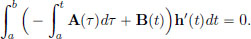
(Only if part). So far we’ve calculated ′(0) and found out that it is the continuous linear transformation L. Now suppose that ′(0) = L = 0, that is, for all h ∈ X, Lh = 0, and so
for all h ∈ C1[a, b] with h(a) = h(b) = 0, 
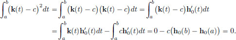
We would now like to use the technical result (Lemma 3.1) we had shown. So we rewrite the above integral and convert the term in the integrand which involves h, into a term involving h′, by using integration by parts:
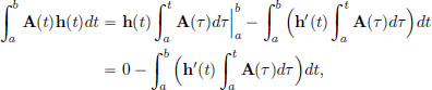
because h(a) = h(b) = 0. So for all h ∈ C1[a, b] with h(a) = h(b) = 0, we have
By Lemma 3.1, 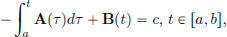 for some constant c.
By differentiating with respect to t, we obtain

(If part). Now suppose that x∗ satisfies the Euler-Lagrange equation, that is, A(t) − B′(t) = 0 for all t ∈ [a, b]. For h ∈ X, we have

Thus for all h ∈ X,
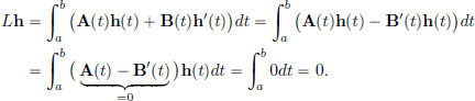
Consequently, ′(0) = L = 0
Let (1)S = {x ∈ C1[a, b] : x(a) = ya, x(b) = yb},
(2)
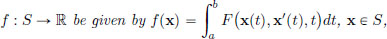
(3)f : S → R be given by 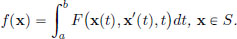
Then we have:
(a)If x∗ is a minimiser of f, then it satisfies the Euler-Lagrange equation:

(b)If f is convex, and x∗ ∈ S satisfies the Euler-Lagrange equation, then x∗ is a minimiser of f .
Proof. Let X := {x ∈ C1[a, b] : x(a) = 0, x(b) = 0}, and : X → R be given by (h) = f(x∗ + ), h ∈ X. Then is well-defined.
(a)We claim that has a minimum at 0 ∈ X. Indeed, for h ∈ X, we have

So by Theorem 3.2, page 126, ′(0) = 0. From Theorem 3.5, page 134, it follows that x∗ satisfies the Euler-Lagrange equation.
(b)Now let f be convex and x∗ ∈ S satisfy the Euler-Lagrange equation. By Theorem 3.5, it follows that ′(0) = 0. The convexity of f makes convex as well. Indeed, if h1, h2 ∈ X, and α ∈ (0, 1), then
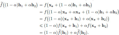
Recall that in Theorem 3.4, page 132, we had shown that for a convex function, the derivative vanishing at a point implies that that point is a minimiser for the function. Since is convex, and because ′(0) = 0, 0 is a minimiser of . We claim that x∗ is a minimiser of f.
Indeed, if x ∈ S, then x = x∗ + (x – x∗) = x∗ + h, where h := x – x∗ ∈ X.
Hence

This completes the proof.
Let us revisit Example 0.1, page viii, and solve it by observing that it falls in the class of problems considered in the above result.
Example 3.7. Recall that S := {x ∈ C1[0, T] : x(0) = 0 and x(T) = Q}, so that we have a = 0, b = T, ya = 0 and yb = Q. The cost function f : S → R was given by

where a, b, Q > 0 are constants, and F : R3 → R is given by

So this problem does fall into the class of problems covered by Corollary 3.1. In order to apply the result to solve this problem, we compute

The Euler-Lagrange equation for x∗ ∈ S is:
that is, 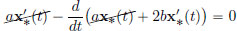 for all t ∈ [0, T]. Thus

By the Fundamental Theorem of Calculus, it follows that there is a constant A such that x′(t) = A, t ∈ [0, T], and integrating again, we obtain a constant B such that x∗(t) = At + B, t ∈ [0, T]. But since x∗ ∈ S, we also have that x∗(0) = 0 and x∗(T) = Q, which we can use to find the constants A, B: A · 0 + B = 0, and A · T + B = Q so that B = 0 and A = Q/T. Consequently, by part (a) of the conclusion in Corollary 3.1, we know that if x∗ is a minimiser of f, then
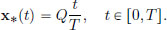
On the other hand, we had checked in Example 3.6 that f is convex. And we know that the x∗ given above satisfies the Euler-Lagrange equation. Consequently, by part (b) of the conclusion in Corollary 3.1, we know that this x∗ is a minimiser. So we have shown, using Corollary 3.1, that
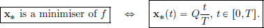
So we have solved our optimal mining question.
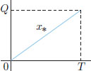
And we now know that the optimal mining operation is given by the humble straight line!
Exercise 3.13. (Euclidean plane).
Let P1 = R2 with ||(x, t)||1 :=  for (x, t) ∈ P1.
Set S := {x ∈ C1[a, b] : x(a) = xa, x(b) = xb}.
Given x ∈ S, the map  is a curve in the Euclidean plane P1, and we define its arc length by
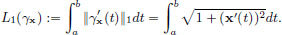
Show that the straight line joining (xa, a) and (xb, b) has the smallest arc length.
Exercise 3.14. (Galilean spacetime).
Let P0 = R2 with ||(x, t)||0 :=  for (x, t) ∈ P0.
Set S := {x ∈ C1[a, b] : x(a) = xa, x(b) = xb}.
Given x ∈ S, the map  is a curve in the Euclidean plane P0, and we define its arc length by
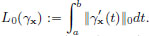
Show that all the curves γx joining (xa, a) and (xb, b) have the same arc length. (If we think of P0 as the collection of all events (=“here and now”), with the coordinates provided by an “inertial frame3” choice, then this arc length is the pre-relativistic absolute time between the two events (xa, a) and (xb, b).)
Exercise 3.15. (Minkowski spacetime).
Let P−1 = R2 with ||(x, t)||−1 := for (x, t) ∈ P0.
Set S := {x ∈ C[a, b] : x(a) = xa, x(b) = xb, for all a t b, |x′(t)| < 1}.
Given x ∈ S, the map  is a curve in the Euclidean plane P−1, and we define its arc length by
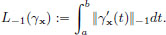
Show4 that among all the curves γx joining (xa, a) and (xb, b), the straight line has the largest(!) arc length.
(P−1 can be thought of as the special relativistic spacetime of all events, with the coordinates provided by an “inertial frame” choice. Then the arc length L(γx) is the proper time between the two events (xa, a) and (xb, b), which may be thought of as the time recorded by a clock carried by an observer along its worldline γx. The fact that the straight line has the largest length accounts for the aging of the travelling sibling in the famous Twin Paradox: Imagine two twins, say Seeta and Geeta, who are separated at birth, event (0, 0) in an inertial frame, and meet again in adulthood at the event (0, T). Seeta, the meek twin, doesn’t move in the inertial frame, described by the straight line γS joining the events (0, 0) and (0, T). Meanwhile, the other feisty twin, Geeta, travels in a spaceship (never exceeding the speed of light, 1), with a worldline given by γG, starting at (0, 0), and ending to meet the twin at (0, T) as shown.
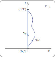
There is no longer any surprise that Seeta has aged far more than Geeta, thanks to our inequality that L(γG) < L(γS). Resting is rusting!)
Exercise 3.16. (Euler-Lagrange Equation: vector valued case).
The results in this section can be generalised to the case when f has the form

where (ξ1, ···, ξn, η1, ···, ηn, τ) F(ξ1, ···, ξn, η1, ···, ηn, τ) : R2n+1 → R is a function with continuous partial derivatives of order 2, and x1, ···, xn are n continuously differentiable functions of the variable t ∈ [a, b].
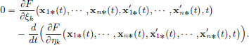
Then following a similar analysis as before, we obtain n Euler-Lagrange equations to be satisfied by the minimiser (x1∗, ···, xn∗): for t ∈ [a, b], and k ∈ {1, ···, n},
Let us see an application of this to the planar motion of a body under the action of the gravitational force field (planet around the sun).
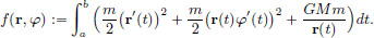
If x1(t) = r(t) (the distance to the sun), and x2(t) = φ(t) (radial angle), then the function to be minimised is
Show that the Euler-Lagrange equations give

(The latter equation shows that the angular momentum, L(t) := mr(t)2 φ′(t), is conserved, and this gives Kepler’s Second Law, saying that a planet sweeps equal areas in equal times.)
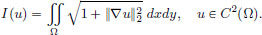
Exercise 3.17. (Euler-Lagrange Equation: several independent variables). Suppose that Ω ⊂ Rd is a “region” (an open, path-connected set), and that

is a given C2 function (called the Lagrangian density).
We are interested in finding u ∈ C1(Ω) which minimise I : C1(Ω) → R given by
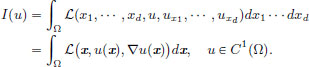
(Here subscripts indicate respective partial derivatives: for example, 
It can be shown that a necessary condition for u to be a minimiser of I is that it satisfies the Euler-Lagrange equation below:
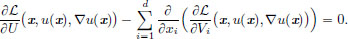
(Note that the Euler-Lagrange equation above is now a Partial Differential Equation (PDE), rather than the Ordinary Differential Equation (ODE) we had met in Theorem 3.5, page 134.)
Let us consider examples of writing the Euler-Lagrange equation.
(1)(Minimal area surfaces).
Consider a smooth surface in R3 which is the graph of (x, y) u(x, y) defined on an open set Ω ⊂ R2.
The area of the surface is given by:
Show that if u is a minimiser, then u must satisfy the PDE

Verify that the following solve this PDE: 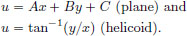
Also, in the case of the helicoid, show that a parametric representation of the surface is given by x(s, t) = s · cos t, y(s, t) = s · sin t, z(s, t) = t, by setting  and t = tan−1(y/x). Plot the surface5 with Maple using:

(2)(Wave equation).
Consider a vibrating string of length 1, whose ends are fixed.
If u(x, t) denotes the displacement at position x and time t, where 0 x 1, then the potential energy at time t is given by
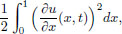
and the kinetic energy is 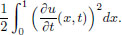
For u : [0, 1] × [0, T] → R, set

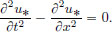
Prove that if u∗ minimises I, then it satisfies the wave equation
Show that if f : R → R is
-twice continuously differentiable,
-odd (f(x) = −f(–x) for all x ∈ R), and
-periodic with period 2 (that is, f(x + 2) = f(x) for all x ∈ R),
then u given by 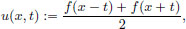 is such that
-it solves the wave equation,
-with the boundary conditions u(0, ·) = 0 = u(1, ·) and
-the initial conditions u(·, 0) = f (position) and  (velocity).
Interpret the solution graphically.
The aim of this section is to apply the Euler-Lagrange equation to illustrate some basic ideas in classical mechanics. Also, this brief discussion will provide some useful background for discussing Quantum Mechanics later on, as an application of Hilbert spaces and their operators.
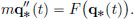
Newtonian Mechanics. Consider the motion t q∗(t) of a classical point particle of mass m along a straight line. Here q∗(t) denotes the position of the particle at time t.
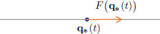
Then the evolution of q∗ is described by Newton’s Law, which says that the “mass times the acceleration equals the force acting”, that is, if F(x) is the force at position x, then
Together with the particle’s initial position q∗(ti) = qi, and initial velocity  (ti) = vi, the above equation determines a unique q∗.
Principle of Stationary Action. An alternative formulation of Newtonian Mechanics is given by the “Principle of Stationary6 Action”, which is more useful because it lends itself to generalisations for other types of physical situations, for example in describing the electromagnetic field (when there are no particles). In that sense it is more fundamental as it provides a unifying language.
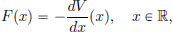
First, let us define the potential V : R → R as follows. Choose any x0 ∈ R, and set
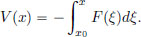
V is thought of as the work done against the force to go from x0 to x. (Because of the fact that x0 was chosen arbitrarily, the potential V for a force F is not unique. By the Fundamental Theorem of Calculus, we have
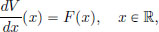
and so it can be seen that if V,  are potentials for F, then as
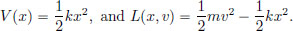
there is a constant c ∈ R such that (x) = V(x) + c, x ∈ R.) We define the kinetic energy of the particle at time t as

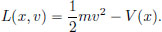
Consider for q ∈ C1[ti, tf] with q(ti) = xi and q(tf) = xf, the action
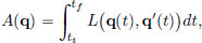
where L is called the Lagrangian, given by L(x, v) =  mv2 − V(x).
Note that along an imagined trajectory q of a particle,

The Principle of Stationary Action in Classical Mechanics says that the motion q∗ of the particle moving from position xi at time ti to position xf at time tf is such that Ã′(0) = 0, where à : X → R is given by

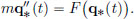
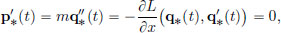
By Theorem 3.5, page 134, the Euler-Lagrange equation is equivalent to Ã′(0) = 0, and so the motion q∗ is described by
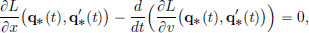
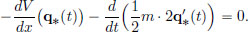
Using 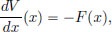 we obtain Newton’s equation of motion,
Here are a couple of examples.
Example 3.8. (The falling stone).
Let x 0 denote the height above the surface of the Earth of a stone of mass m. Then its potential energy is given by V(x) = mgx. Thus

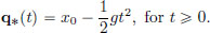
Suppose the stone starts from initial height x0 > 0 at time 0, with initial speed 0. Then the height q∗(t) at time t is described by 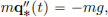 that is,

Using the initial conditions, we obtain 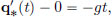 and so
Example 3.9. (The Harmonic Oscillator).
The harmonic oscillator is the simplest oscillating system, where we can imagine a body mass m attached to a spring with spring constant k oscillating about its equilibrium position. For a displacement of x from the equilibrium position of the mass, a force of kx is imparted on the mass by the spring. So
The equation of motion is
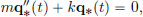
describing the displacement q∗(t) from the equilibrium position at time t. If v0 is the velocity at time t = 0, and the initial position is q∗(0) = 0, then the unique solution is
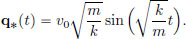
(It can be easily verified that this q∗ satisfies the equation of motion 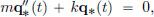 as well as the initial conditions
  and
and 
The maximum displacement is
and the period of oscillation is 
“Symmetries” of the Lagrangian give rise to “conservation laws”:
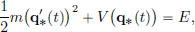
Law of Conservation of Energy. Since the Lagrangian L(x, v) does not depend on t (that is, it possesses “the symmetry of being invariant under time translations”), we will now see that this results in the Law of Conservation of Energy. Define the energy E(t) along q∗ at time t by
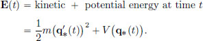
Then we have
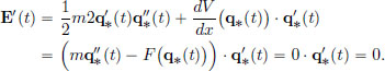
Hence the energy E is constant, that is, it is conserved.
Law of Conservation of Momentum. Now suppose that the Lagrangian does not depend on the position, that is, L(x, v) = l(v) for some function l. Define the momentum p∗t along q∗ at time t by

Then
and so p∗ is constant, that is, the momentum is conserved.
Remark 3.2. (Noether’s Theorem).
The above two results are special cases of a much more general result, called Noether’s Theorem, roughly stating that every differentiable symmetry of the action has a corresponding conservation law. This result is fundamental in theoretical physics. We refer the interested reader to the book [Neuenschwander (2011)].
Example 3.10. (Particle in a Potential Well).
Consider a particle of mass m moving along a line, and which is acted upon by a force
generated by a potential V. The associated Lagrangian is
Suppose that the motion of the particle is described by q∗ for t 0. If

then for all t 0, we have by the Law of Conservation of Energy, that
and so 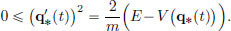 This implies that V(q∗(t)) E. Hence the particle cannot leave the potential well if V(x) → ∞ as x → ±∞.

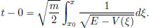
If the velocity of the particle is always positive while moving from initial position x0 at time t = 0 to a position x > x0 at time t, then by integrating,
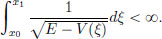
If in this manner, the particle reaches x1, where E = V(x1) (see the previous picture), then we may ask if the travel time t1 from x0 to x1 is finite.
The above expression reveals that t1 < ∞ if and only if
In particular, in the case of the harmonic oscillator, where

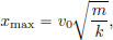
we have that the time of travel from the initial condition x0 to the maximum displacement xmax is finite, and is given by
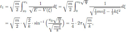
which is, as expected, one-fourth of the period of oscillation.
Hamiltonian Mechanics.
The momentum p∗ is defined by  Since
Since  we have
The Euler-Lagrange equation,  can be re-written as
It turns out that the above two equations can be expressed in a much more symmetrical manner, with the introduction of the Hamiltonian,
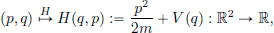
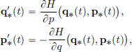
as follows. Note that
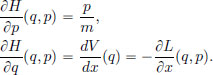
Thus
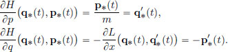
These two equations are equivalent to 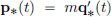 and the Euler-Lagrange equation. The space {(q, p) ∈ R2} is called the phase plane, where the position-momentum pairs live. Each point (q, p) in the phase plane is thought of as a possible state of the particle. Given an initial state (q0, p0), the coupled first order differential equations, describing the evolution of the state, namely the Hamiltonian equations
for t 0, describe a curve t (q∗(t), p∗(t)) in the phase plane, called a phase plane trajectory. The collection of all phase plane trajectories, corresponding to various initial conditions, is called the phase portrait. The following picture shows the phase portrait for the harmonic oscillator.
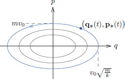
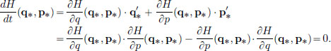
We also observe that the Hamiltonian H, evaluated along a phase plane trajectory t (q∗(t), p∗(t)), is

the energy, which by the Law of Conservation of Energy, is a constant. So the phase plane trajectories are contained in level sets of the Hamiltonian H. Another proof of this constancy of the function H along phase plane trajectories, based on the Hamiltonian equations, is given below (where we have suppressed writing the argument t):
This sort of a calculation can be used to calculate the time evolution of any “observable” (q, p) f(q, p) along phase plane trajectories in the phase plane, as explained in the next paragraph.
Poissonian Mechanics.
All the (mechanical) physical characteristics are functions of the state. For example in our one-dimensional motion of the particle, the coordinate functions (q, p) q and (q, p) p give, for a state (q, p) of the particle, the position, respectively the momentum, of the particle. Similarly,

gives the energy. Motivated by these considerations, we take

as the collection of all observables.
We now introduce a binary operation {·, ·} : C∞;(R2) × C∞(R2) → C∞(R2), which is connected with the evolution of the mechanical system.
Given two observables F and G in C∞(R2), define the new observable {F, G} ∈ C∞(R2), called the Poisson bracket of F, G, by

The Poisson bracket can be used to express the evolution of an observable F. Suppose that our particle moving along a line, evolves along the phase plane trajectory (q∗, p∗) in the phase plane according to Hamilton’s equations for a Hamiltonian H. Then the evolution of the observable F ∈ C∞(R2) along the trajectory (q∗, p∗) is given by (again suppressing t):
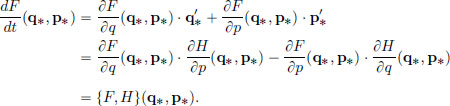
In particular, if {F, H} = 0 (as for example is the case when F = H!), then F is a conserved quantity.
It can be shown that C∞(R2) forms a Lie algebra with the Poisson bracket, that is, the following properties hold:
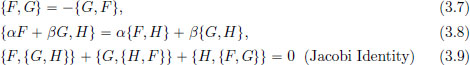
for α, β ∈ R and any F, G, H ∈ C∞(R2). (H may not be the Hamiltonian!)
We will see in the next chapter, that the role of the Poisson bracket in classical mechanics,

of observables F, G ∈ C∞(R2), is performed by the commutator

of observables A, B (which are operators on a Hilbert space H) in quantum mechanics.
Exercise 3.18. Prove (3.7)-(3.9).
Exercise 3.19. (Position and Momentum).
Let Q ∈ C∞(R2) be the position observable, 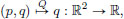 and P ∈ C∞(R2) be the momentum observable
 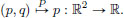 Show that {Q, P} = 1.
1See for example [Luenberger (1969)].
2In fact, not even a “local” minimiser because ||x − 0||∞ = α can be chosen as small as we please.
3A coordinate system is inertial if particles which are “free” that is, not acted upon by any force, move in straight lines with a uniform speed.
4Here we tacitly ignore the fact that the set S doesn’t quite have the form that we have been considering, since we have the extra constraint |x′(t)| < 1 for all ts. Despite this extra condition, a version of Corollary 3.1 holds, mutatis mutandis, with an appropriately adapted proof: instead of X := {h ∈ C1[a, b] : h(a) = 0 = h(b)}, we work in the open subset X0 := {h ∈ X :|h′(t)| < 1 for all t ∈ [a, b]} of X. We won’t spell out the details here, but we simply use the Euler-Lagrange equation in this exercise.
5This surface has the least area with a helix as its boundary.
6It is standard to use “Least” rather than “Stationary” because in many cases the action is actually minimised.