Chapter 6

A glimpse of distribution theory

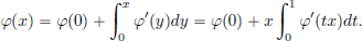
In this last chapter of the book, we will see a generalisation of functions

and their ordinary calculus to “distributions” or “generalised functions”. These distributions will be “continuous linear functionals on the vector space of test functions D(R^d)”:

Why study distributions? We list three main reasons:

(1)To mathematically model the situation when one has an impulsive force (imagine a blow to an object which changes its momentum, but the force itself is supposed to act “impulsively”, that is the time interval when the force is applied is 0!). Similar situations arise in other instances in mathematics and the applied sciences.

(2)To develop a calculus which captures more general situations than the classical case. For example, what is the derivative of |x| at x = 0?
It will turn out that this is also useful to talk about weaker notions of solutions of Partial Differential Equations (PDEs).

(3)To extend the Fourier transform theory to functions that may not be absolutely integrable. For example, what1 is the Fourier transform of the constant function 1?

It turns out that the theory of distributions solves all of these three problems in one go. This seems like a miracle, and naturally there is a price to pay. The price is that everything classical is now replaced by a weaker notion. Nevertheless this is useful, since it is often sufficient for what one wants to do. An example is that, as opposed to functions on R, which have a well-defined value at every point x ∈ R, we can no longer talk about the value of a distribution at a point of R.

Let us elaborate on reason (2) above, in the context of PDEs. An example we met earlier in Exercise 3.17, page 143, is that of the wave equation (which describes the motion of a plucked guitar string), and we had checked that for a twice continuously differentiable f

gives a solution with the initial condition described by f (and zero initial velocity). However, when we pluck a guitar string, the initial shape needn’t be C², and in fact, it could have a corner like this:

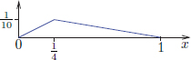
Nature of course doesn’t care about the lack of classical differentiability of our candidate solution to the PDE model, and produces a travelling wave solution, with time snapshots that look like the ones shown in Figure 6.1. We must have at sometime witnessed choppy waves on the surface of the sea on a windy day.

Thus it is desirable to weaken the notion of differentiability, to allow for such (classically) non-differentiable solutions to nevertheless serve as solutions to the wave equation. We will see that such a weaker notion is provided by viewing our function as a more general object, namely a distribution, and with its weaker distributional calculus, the wave equation will be satisfied!

So with this motivation, we will begin to learn the very basics of the theory of distributions in this chapter, and also see a glimpse of its applications to PDEs. For a firm foundation of the theory of distributions, one needs preliminaries on topological vector spaces². Here we will adopt a “working” approach, in which we will learn rigorous, but (seemingly) ad hoc definitions about continuity and convergence, in the spaces related to distributions. We will make a few remarks that will serve as a guide to the reader who wishes to delve into the subject deeper.

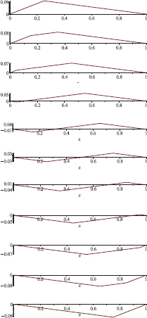
Fig. 6.1 Time snapshots of a plucked guitar string.

We first make a brief historical remark about the story of the development of distributions. The prime example of a distribution, the “delta function” δ_a, was introduced3 in the 1930s in order to do quantum mechanical computations (as eigenstates of the position operator). However, a firm mathematical foundation for this and other generalised functions had to wait till the 1950s when the French mathematician Laurent Schwartz introduced the concept of distributions and developed its theory. For this, he was awarded the Fields medal.

6.1Test functions, distributions, and examples

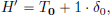
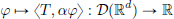
It will turn out that distributions are functionals on a vector space, namely the vector space of “test functions”. Just like a function f : R^d → C can be evaluated at a point x ∈ R^d giving a number f(x), we will see later on that a distribution T on R^d can be “tested against” a test function φ, giving a number 〈T, φ〉. Let us first begin by describing this vector space D(R^d) of test functions.

Definition 6.1. (Test function). A test function φ : R^d → C is an infinitely differentiable function, for which there exists a compact set, outside which φ vanishes. The set of all test functions is denoted by D(R^d). Equipped with pointwise operations, D(R^d) is a vector space. Thus:

Example 6.1. Let φ : R → R be given by

We claim that φ is a test function, that is, it is an element of D(R).

It is clear that φ vanishes outside the compact interval [−1, 1].

Moreover, it is also infinitely many times differentiable:

Indeed, it can be seen that the function f : R → R given by

is clearly infinitely many times differentiable outside 0, and also

showing that f is infinitely many times differentiable everywhere on R. (See Exercise 6.1 where the details are spelt out.)

The graph of f is shown in the following picture.

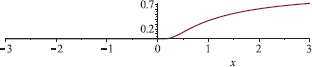
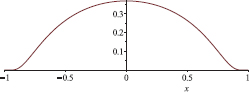
The function φ is just the composition of f with the polynomial x 1 − x².

The picture below shows the graph of φ.

Similarly, we could have composed f with the function

and obtained a function in D(R^d) that is C^∞ and is zero outside the closed unit ball B(0, 1) := {x ∈ R^d : ||x||₂ 1} in R^d. Note that as B(0, 1) is closed and bounded in R^d, it is compact.

Based on the above example, it might seem that test functions are rather special, and are few and far between. But let us note that whenever we have a φ ∈ D(R^d), then for every λ > 0 and every a ∈ R^d, also the functions

belong to D(R^d). Moreover, it is easy to see that D(R^d) is closed under partial differentiation. (In the following, it will be convenient to introduce the following notation: if k = (k₁, · · · , k_d) is a multi-index of nonnegative integers, then

In this notation, we have: φ ∈ D(R^d) D^kφ ∈ D(R^d) for all k.) By taking linear combinations, we see that we thus get a huge abundance of functions in D(R^d).

Exercise 6.1. (∗)(A C^∞ function which is not analytic.)

(1)Suppose that f : R → R is continuous on R, continuously differentiable on R_∗ := R\{0}, and such that f′(x) exists.

Show that f is continuously differentiable on R.

(2)Let f : R → R be n − 1 times continuously differentiable, n times continuously differentiable on R_∗, and such that f⁽ⁿ⁾(x) exists.

Show that f is n times continuously differentiable on R.

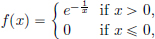
(3)Let f : R → R given by

Show that f is infinitely many times differentiable.

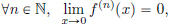
Hint: Using induction on n, show that for x > 0, f⁽ⁿ⁾(x) = R_n(x)f(x), where R_n is a rational function. Conclude that x⁻ⁿ f(x) = 0.

Exercise 6.2. Solve = 0 in D(R²).

Exercise 6.3. Show that {Φ′ : Φ ∈ D(R)} = {φ ∈ D(R) : φ(x)dx = 0} =: Y.

Also, show that if φ ∈ Y, then the Φ ∈ D(R) such that Φ′ = φ is unique.

Definition 6.2. (Convergence in D(R^d)).

We say that a sequence (φ_n)_n∈N converges to φ in D(R^d) if

(1)there exists a compact set K ⊂ R^d such that all the φ_n vanish outside K, and

(2)φ_n converges uniformly4 to φ, and for each multi-index k, D^kφ_n converges uniformly to D^kφ.

We then simply write .

Remark 6.1. (Topology on D(R^d)).

It turns out that D(R^d) is a topological space with a certain topology (with a collection of open sets denoted by, say O), allowing one to then talk about convergent sequences in this topology given by O. It can be shown that (φ_n)_n∈N converges to φ in the topological space (D(R^d), O) if and only if it converges in the above sense. See for example [Bremermann (1965), Appendix 1, pages 37–40].

Exercise 6.4. Let (φ_n)_n∈N be a sequence in D(R) such that for each n ∈ N,

From Exercise 6.3, it follows that for each n ∈ N, there exists a unique Φ_n ∈ D(R), such that . Suppose moreover that . Prove that .

Now that we have a vector space D(R^d), with a topology, one can talk about continuous linear transformations D(R^d) from C, and these are called distributions. The precise definition is as follows.

Definition 6.3. (Distribution).

A distribution T on R^d is a map T : D(R^d) → C such that

(1)(Linearity) For all φ, ψ ∈ D(R^d) and all α ∈ C,

(2)(Continuity) If , then T(φ_n) → T(φ).

The set of all distributions is denoted by D′(R^d).

With pointwise operations, D′(R^d) is a vector space.

We will usually denote T(φ) for φ ∈ D(R^d), by 〈T, φ〉.

Remark 6.2. It is enough to check the continuity requirement with φ = 0, since from the linearity of T, it follows that T(φ_n) − T(φ) = T(φ − φ_n), and it is clear that if and only if .

Remark 6.3. It can be shown that a linear transformation from D(R^d) to C is continuous, with respect to the aforementioned (Remark 6.1) topology on D(R^d) given by O, if and only if it is continuous in the above sense (given by item (2) in the above definition). See for example [Rudin (1991), Theorem 6.6 on page 155].

When first encountered, distributions may seem very strange objects indeed, far removed from the world of ordinary functions that we are used to. But now we’ll see that practically all functions one meets in practice, can be viewed as distributions. This will enable us later, to apply the distributional calculus we develop, also to functions (by viewing them as distributions), and it will be in this sense, that we’ll be able check that even with a non-C² function f, the u given by (6.1) satisfies the wave equation.

Example 6.2. ((R^d) functions are distributions.)

Let f : R^d → C be a locally integrable function (written f ∈ (R^d), that is, for every compact set K,

Here dx stands for the volume element dx₁ · · · dx_d in R^d.

Then f defines a distribution T_f as follows:

The integral exists since φ is bounded and zero outside a compact set, and so we are actually integrating over a compact set.

It is also easy to see that T_f is linear.

Continuity: Let . Then there is a compact set K such that all φ_n, n ∈ N, vanish outside K. We have

since φ_n converges to 0 uniformly on K (the derivatives of φ_n play no role here). Consequently, T_f ∈ D′(R^d).

Distributions T_f, where f is locally integrable, are called regular distributions. An example of a function f ∈ (R) is the Heaviside function, whose graph is displayed in the picture on the left below.

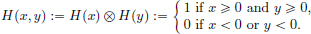
The Heaviside5 function H is given by

The value H(0) of the function H at x = 0 can be arbitrarily assigned, since for any φ ∈ D(R), the value of the integral

won’t change, no matter what choice we make for H(0)! So the distribution T_H will be the same, irrespective of what number we set H(0) to be.

We denote the distribution T_H simply by the symbol H from now on.

Theorem 6.1. The following are equivalent for f, g ∈ (R^d) :

(1)T_f = T_g.

(2)For almost all x ∈ R^d, we have f(x) = g(x).

In particular, if f and g are continuous, then T_f = T_g if and only if f = g.

Theorem 6.1 means that the map f T_f, from (R^d) (which is the space of equivalence classes of locally integrable functions that are equal almost everywhere), to D′(R^d), is injective. In practice, one identifies (the equivalence class of) f ∈ (R^d) with the distribution T_f, and one considers the map f T_f : (R^d) → D′(R^d) as an inclusion: (R^d) ⊂ D′(R^d). So just like we identify each integer as a rational number, we may think of all locally integrable functions as distributions. Since the map f T_f is linear (that is, T_f+g = T_f + T_g and T_αf = αT_f), this identification respects addition and scalar multiplication. As the space C(R^d) of continuous functions can be considered as a subspace of (R^d) (two continuous functions on R^d that are equal almost everywhere are identical), we get the following inclusions:

We won’t include the proof of Theorem 6.1 here. The interested reader is referred to [Schwartz (1966), Theorem 2, page 74]. The following example shows that the inclusion (R^d) ⊂ D′(R^d) is strict, that is, not all distributions are regular.

Example 6.3. (Dirac delta distribution).

The distribution δ ∈ D′(R^d) is defined by

More generally, one defines, for a ∈ R^d, a distribution δ_a by

It is evident that δ_a is linear and continuous on D(R^d), that is, it is a distribution.

The delta distribution is not regular: there is no function f ∈ (R^d) such that δ_a = T_f. Nevertheless, in a huge amount of literature, one encounters a manner of writing that suggests that δ_a is a regular distribution. In place of 〈δ, φ〉, one writes

One then talks about delta “functions” instead of delta distributions. This is of course incorrect (see Exercise 6.5 below), but in some sense useful if one wants to do formal manipulations in order to guess answers, or in order to get physical insights etc.

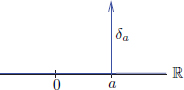
With this fallacious viewpoint, one often depicts the “graph of δ_a ∈ D′(R)” as a spike positioned at a, with the intuitive feeling that the “δ_a function is everywhere 0, but is infinity at x = a, and has integral over R equal to 1”!

Exercise 6.5. Show that there is no function δ : R → R such that for all a > 0:

(1)δ is Riemann integrable on [−a, a], and

(2)for every C^∞ function φ vanishing outside [−a, a], δ(x)φ(x)dx = φ(0).

Example 6.4. pv.

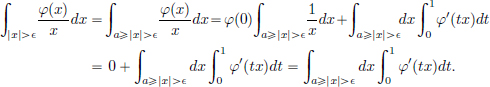
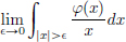
Although the function x (defined almost everywhere on R) is not locally integrable, nevertheless one can associate a distribution T with this function: for all φ ∈ D(R),

(pv stands for “principal value”).

That the limit above exists, and that T defines a distribution can be seen as follows. Suppose that φ = 0 on R\[−a, a], where a > 0. We have:

Since 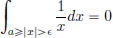, we have

Thus exists, and .

Continuity: Let , and suppose that a > 0 is such that for all n ∈ N, φ_n = 0 outside [−a, a]. Then |〈T, φ_n〉| 2a · .

This distribution is denoted by pv, so that .

(In quantum mechanics (perturbation theory) one encounters

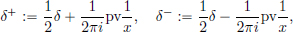
having the property δ = δ ⁺ + δ⁻.)

Exercise 6.6.

(1)For φ ∈ D(R), set 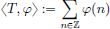. Show that T ∈ D′(R).

(2)Give an example of a sequence of test functions (φ_n)_n∈N such that:

(a) uniformly, and for all k ∈ N, also uniformly, but

(b).

Hint: Consider a sequence of test functions of the type with an appropriate choice of φ.

(3)Does the construction in part (2) contradict our conclusion in (1) that T is a distribution?

6.2Derivatives in the distributional sense

We will now develop a calculus for distributions.

Let us first consider the case when d = 1.

Definition 6.4. (Distributional derivative, d = 1). Let T ∈ D′(R).

Then the distributional derivative 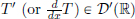of T is defined by

Note that if φ ∈ D(R), then clearly φ′ ∈ D(R). So the right-hand side above is well defined.

Moreover, the map φ −〈T, φ′〉 is linear: for all φ, ψ ∈ D(R) and α ∈ C,

Continuity of T′: If , then also , and so . Thus T′ ∈ D′(R).

Q.Is distributional differentiation an extension of classical differentiation?

A.Yes. The result below (Lemma 6.1) shows that our new definition is a sensible generalisation from the classical case: If we have a continuously differentiable function, and if we choose to put on our “distributional glasses”, then the distribution we get, by distributionally differentiating the corresponding regular function, is a regular distribution corresponding to the classical derivative.

Lemma 6.1. If f ∈ C¹(R), then (T_f)¹ = T_f′.

Proof. Let φ ∈ D(R) be such that it vanishes outside [a, b]. Then using integration by parts,

(Here we have used that φ, φ′ are zero outside [a, b], and φ(a) = φ(b) = 0.) This completes the proof.

The above result means that whenever one identifies the function f with the distribution T_f, then the two possible interpretations of the derivative which arise – the classical sense versus the new distributional sense – coincide. In fact, this is the motivation behind our definition of the distributional derivative given in Definition 6.4.

The next example shows that now, endowed with our notion of the distributional derivative, we can differentiate functions which we couldn’t earlier (albeit only in the distributional sense).

Example 6.5. (H′ = δ).

Let us show that the Dirac distribution is the distributional derivative of regular distribution corresponding to the Heaviside function H ∈ (R). For any test function φ ∈ D(R), we know that φ(x) = 0 for all sufficiently large x, and so

and so H′ = δ.

Example 6.6. (Dipole).

The derivative δ′ of δ, is called the dipole, and is given by

for all φ ∈ D(R).

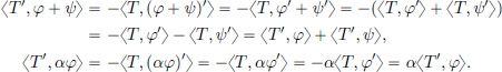
In Example 6.5, the classical derivative of H for the regions x < 0 and x > 0 is equal to 0 everywhere, and it is right to think philosophically that the δ appeared owing to the jump in the values of H from 0 to 1 as x went from negative to positive values.

So we can write

where T₀ is the regular distribution corresponding to the zero function 0, and the coefficient 1 multiplying δ₀ is the “jump” in the value of H at 0. This is no coincidence, and the observation can be generalised as follows.

Proposition 6.1. (Jump Rule).

Let f be continuously differentiable on R except at the point a ∈ R, where the limits f(a+), f(a−), f′(a+), f′(a−) exist.

Then f, f′ are locally integrable, and

We think of f(a+) − f(a−) as the jump in f at the point a. One can formulate this result by saying:

The derivative of f in the sense of distributions is

the classical derivative plus δ_a times the jump in f at a.

Proof. Let φ ∈ D(R), and suppose that φ is 0 outside [α, β], and that a ∈ [α, β]. Then

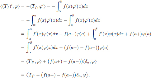
Example 6.7. (|x|′ = 2H − 1). In the sense of distributions,

Indeed, the jump in |x| at x = 0 is |x| − |x| = 0 − 0 = 0.

For x ≠ 0, |x| is differentiable with derivative 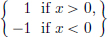= 2H(x)−1.

Finally, (2H(x) − 1) = 1 and (2H(x) − 1) = −1.

So by the Jump Rule, (T_|x|)′ = T_2H−1, or briefly |x|′ = 2H − 1 in the sense of distributions.

Remark 6.4. This result can be extended to the case when f is continuously differentiable everywhere except for a finite number of points a_k, and at these points a_k, the function satisfies the same assumptions as stipulated above. This then leads to

The proof is analogous.

In fact the result even extends to the case when f has infinitely many, but locally finite, jump discontinuities: in any compact interval, one finds only finitely many discontinuities. The sum on the right-hand side is the distribution defined by

where, for a given test function φ, only finitely many terms on the right-hand side are nonzero.

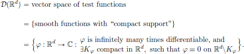
Example 6.8. . See the pictures below.

Here · is the greatest integer function, that is, for x ∈ R, x is the greatest integer less than or equal to x.

Exercise 6.7.

Show that H(x) cos x = −H(x) sin x + δ and H(x) sin x = H(x) cos x.

One can define higher order distributional derivatives by iteratively setting T⁽ⁿ⁾ := (Tⁿ⁻¹)′ for n 2.

Exercise 6.8. (Fundamental Solution to the 1D Laplace equation).

Show that the equation is satisfied by .

Exercise 6.9. (Zero distributional derivative implies constancy.)

The aim of this exercise is to show that if T ∈ D′(R), and T′ = 0, then there exists a constant c such that T = T_c, the regular distribution associated with the constant function taking value c everywhere on R. To prove this result, we will proceed as follows.

(1)Let V be a complex vector space. If ℓ, L ∈ L(V, C) are such that ker ℓ ⊂ ker L, then there exists a constant c ∈ C such that L = cℓ.

Hint: If v₀ ∈ V is such that ℓ(v₀) ≠ 0, then show that every vector v ∈ V can be decomposed as v = c_vv₀ + w for some c_v ∈ C and some w ∈ ker ℓ.

(2)Prove, using part (1) and Exercise 6.3, page 232, that if the derivative of the distribution T is zero, then T must be constant.

Exercise 6.10. Show that if T ∈ D′(R), then there exists an S ∈ D′(R) such that S′ = T. Moreover, show that such an S is unique up to an additive constant.

Hint: Fix any φ₀ ∈ D(R)\{0} which is nonnegative everywhere. For ψ ∈ D(R),

belongs to the subspace Y of D(R) from Exercise 6.3, page 232.

Hence there exists a unique Φ ∈ D(R) such that Φ′ = φ. Set 〈S, ψ〉 = −〈T, Φ〉.

Exercise 6.11. Show that for all n ∈ N, δ⁽ⁿ⁾ ≠ 0.

Exercise 6.12. Show that {δ, δ′, · · · , δ⁽ⁿ⁾, · · ·} is linearly independent in D′(R).

When d > 1, the definition of the distributional derivative is analogous.

Definition 6.5. (Distributional partial derivatives).

For T ∈ D′(R^d), the ith-partial derivative of T, 1 i d, is defined by

Exercise 6.13. Show that for all T ∈ D′(Rd) and all i, j, .

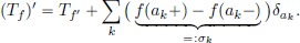
Exercise 6.14. The Heaviside function in two variables, H : R² → R, is defined by

(That is, H is the indicator function 1_[0,∞)² of the “first quadrant”.)

Show that .

Exercise 6.15. (Fundamental solution of the Laplacian on R²).

Verify that , where and .

Remark 6.5. (Sobolev spaces).

There exist Hilbert spaces analogous to the spaces Cⁿ[a, b] defined by:

equipped with the norm || · ||_n defined by:

where || · ||₂ denotes the L² norm. This norm is induced by the inner product

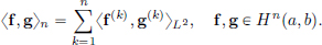
For example: H¹(a, b) = {f ∈ L²(a, b) : f′ ∈ L²(a, b)} and

Since f merely belongs to L²(a, b), we are aware that f^(k) may not have any meaning in general, and so one ought to make the definition precise. This can be done with the theory of distributions. The space Hⁿ(a, b) is the space of functions f ∈ L²(a, b) such that f′, · · · , f⁽ⁿ⁾, defined in the sense of distributions, belong to L²(a, b). Then it can be showed that the space Hⁿ(a, b) is a Hilbert space. The Sobolev spaces Hⁿ(a, b) are named after the Russian Mathematician Sergei Sobolev.

6.3Weak solutions

A function satisfying a PDE in the sense of distributions will be called a weak solution to a PDE.

Example 6.9. Let u(x, t) := H(t)e^x. Then u is locally integrable.

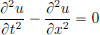
We’ll show that u is a weak solution of the PDE .

We have for all φ ∈ D(R²) that

and so in the sense of distributions.

The following picture shows the graph of this u.

Far from being a classical solution (for which we would want u ∈ C¹) to the PDE, we see that u isn’t even continuous! Nevertheless we accept it as a solution to PDE, since it satisfies the PDE, albeit in the weak sense.

Remark 6.6. (Other notions of weak solutions). Besides distributional solutions, there are other notions too of weak solutions in PDE theory, for example “viscosity solutions” (which are natural in certain contexts, such as the Hamilton-Jacobi equation for optimal control).

Remark 6.7. (Why are weak solutions important?) Weak solutions are important, since as mentioned before, many initial/boundary value problems for PDEs encountered in real world may not possess sufficiently smooth solutions, but only weak solutions, which should not be dismissed. We will see two examples below.

Another reason is “theoretical”: even when there exist classical solutions, it might be easier to find/show the existence of distributional solutions first, and then show later that the solution is in fact sufficiently smooth (and such results are called “regularity results”).

Weak solution to the transport equation

The transport equation is given by

where f is the initial condition, and c ∈ R is a constant.

This equation arises for instance when one models fluid flow6.

It is easy to check that if f ∈ C¹, then a solution is given by

Indeed, u(x, 0) = f(x + c · 0) = f(x + 0) = f(x), and

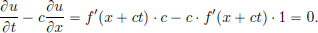
But now, we’ll show that even when f ∈ (R), the same formula, namely u(x, t) := f(x + ct), still gives a solution u to the transport equation. The only change is that it will be a weak solution, that is, the PDE will be satisfied in the “distributional sense”. To see this, let φ ∈ D(R²). Then:

Hence to prove our claim, it must be shown that the above integral is zero. To do this, we will make the following change of variables⁷:

Recall that for a double integral, one has the following “change of variables” formula under the change of variables given by the map :

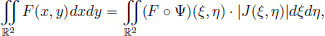
where .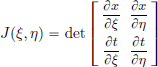

In our case, the derivative of the map is

whose determinant is 1.

We have

Thus

where we have used the Fundamental Theorem of Calculus to simplify the inner integral, and used the fact that φ has compact support to obtain

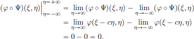
See the following picture.

This shows that u(x, t) := f(x + ct) is indeed a weak solution to the transport equation.

Weak solution to the wave equation

Recall that if f ∈ C²(R), then

is a classical solution to

with the initial condition u(x, 0) = f(x) and with zero initial speed u_t(x, 0) = 0.

Let us now show that even when f is merely locally integrable, u given by (6.5) satisfies the wave equation, but in the sense of distributions. In order to do this, we will use our result from the previous section, where we considered the transport equation.

Let f ∈ (R). Putting c = 1, we have seen that u₊ given by

satisfies, in the sense of distributions, the transport equation

Similarly, putting c = −1, we also see that u₋ given by

is a weak solution to

For any distribution (Exercise 6.13, p. 242). So

Using this observation, we will find a weak solution to the wave equation too. Let u be given by (6.5), and φ ∈ D(R²). Then

To see the equality (∗) in the last line, we note that since φ ∈ D(R²), also

But as

we see that the equality (∗) above holds.

Exercise 6.16. (Weak solution exists, but no classical solution).

Show that 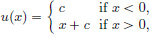is a weak solution of the ODE u′ = H,

where H is the Heaviside function.

6.4Multiplication by C^∞ functions

In general, it is not possible to define the product of two distributions. For example, the product of two locally integrable functions is not in general locally integrable. (f := 1/ is locally integrable, but f² = 1/|x| isn’t!) So the product of two regular distributions in general may not define a distribution.

However, one can define the product of a function α ∈ C^∞(R^d) with a distribution T ∈ D′(R^d) as follows.

Definition 6.6. (Multiplication of a distribution by a smooth function). Let α ∈ C^∞(R^d) and T ∈ D′(R^d). Then αT ∈ D′(R^d) is defined by

Note that if φ ∈ D(R^d), then it is in particular in C^∞(R^d), and so it is clear that αφ is infinitely many times differentiable. Moreover, as φ vanishes outside a compact set, so does αφ. Hence αφ ∈ D(R^d), and the right-hand side makes sense. It is also easy to see that the map

is linear, thanks to the linearity of T. Finally, the continuity of αT can be established by using the multivariable Leibniz Rule for differentiating the product of two functions, which we recall here first:

Leibniz Rule: For a multi-index n = (n₁, · · · , n_d) of nonnegative integers n₁, · · · , n_d, define its

– order |n| by n₁ + · · · + n_d, and

– factorial by n! = n₁! · · · n_d!.

Then the (multivariable) Leibniz Rule states that for every multi-index n := (n₁, · · · , n_d), and functions f, g ∈ C^∞(R^d),

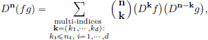
where , and .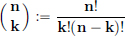

(We will omit the cumbersome, although straightforward, proof of the Leibniz Rule, which proceeds by induction on the order |n| of Dⁿ, and by using the one variable mth derivative formula for the product of two functions.)

Using the Leibniz Rule, it can be seen that if , and if α ∈ C^∞(R^d), then also . Consequently, αT ∈ D′(R^d).

This product of distributions with smooth functions extends the usual pointwise product of a function with a smooth function.

Proposition 6.2. If f ∈ (R^d) and α ∈ C^∞(R^d), then αT_f = T_αf.

Proof. α is bounded on every compact set, and so it follows that αf is locally integrable. For φ ∈ D(R^d), we have

This completes the proof.

The above result means that, whenever we identify as usual the elements of (R^d) with distributions, then the two a priori different manners of forming the product with α lead to the same result.

Example 6.10. One can think of the distribution H(x) cos x as the product of the C^∞ function cos x with the distribution H(x).

Proposition 6.3. The following calculation rules hold.

For T, T₁, T₂ ∈ D′(R^d), α₁, α₂, α, β ∈ C^∞(R^d), we have

(1)α(T₁ + T₂) = αT₁ + αT₂

(2)(α₁ + α₂)T = α₁T + α₂T

(3)(αβ)T = α(βT)

(4)1T = T. (Here 1 ∈ C^∞(R^d) is the constant function R^d ∋ x 1.)

(Thus D′(R^d) is a C^∞(R^d)-module8.)

Proof. All of these follow from the definition of multiplication of distributions by C^∞ functions. For example, to check (3), note that for all φ in D(R^d), 〈(αβ)T, φ〉 = 〈T, (αβ)φ〉 = 〈T, β(αφ)〉 = 〈βT, αφ〉 = 〈(α(βT)), φ〉, proving the claim.

The product rule for differentiation is valid in the same manner as for functions.

Theorem 6.2. (Product Rule). For T ∈ D′(R^d) and α ∈ C^∞(R^d),

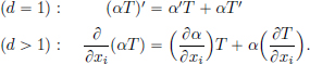
Proof. When d = 1 and φ ∈ D(R), we have (αφ)′ = α′φ + αφ′, and so

The proof is analogous when d > 1. 0

Theorem 6.3. If a ∈ R^d and α ∈ C^∞(R^d), then αδ_a = α(a)δ_a .

Proof. For φ ∈ D(R^d), we have

Example 6.11. (δ_a, a ∈ R, are eigenvectors of the position operator).

Let us recall Exercise 2.35, page 103, where we showed that the position operator Q : D_Q(⊂ L²(R)) → L²(R) given by (Qf)(x) = xf(x), x ∈ R, f ∈ D_Q, has empty point spectrum, and so it has no eigenvectors.

But we can “extend” the operator Q to act not just on functions on R, but also distributions:

Then Q is a linear transformation from D′(R) to itself.

The result in Theorem 6.3 above shows that, for all a ∈ R,

and so δ_a ∈ D′(R), serves as an eigenvector, with corresponding eigenvalue a ∈ R, of the position operator Q ∈ L(D′(R)). (The physicist Paul Dirac used this in 1926 for Quantum Mechanical computations.)

Example 6.12. We have xδ = 0, (cos x)δ = δ, (sin x)δ = 0.

Exercise 6.17. Redo Exercise 6.7, page 241, using the Product Rule.

Exercise 6.18. (Fundamental Solutions).

Show the following, where λ ∈ R, n ∈ N, ω ∈ R\{0}:

Exercise 6.19. Show that if α ∈ C^∞(R), then αδ′ = α(0)δ′ − α′(0)δ. Conclude that xδ′ = −δ.

Exercise 6.20. For T ∈ D′(R), define .

Show that for all T ∈ D′(R), .

(Thus the commutant of , namely

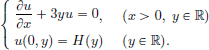
Exercise 6.21. Show that u(x, y) := e^−3yxH(y) is a weak solution of

Exercise 6.22. Show that on D′(R) it is impossible to define an associative and commutative product such that for α ∈ C^∞(R) and T ∈ D′(R), it agrees with Definition 6.6. Hint: Consider the product of δ, x and pv .

Exercise 6.23.

(1)Let T be a distributional solution to the differential equation . Show that T is a classical solution: T = ce^λx. Hint: Differentiate e^−λxT.

(2)(Hypoellipticity9 of
Let f ∈ C^∞(R), and T ∈ D′(R) be a solution to

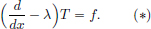
Show that T is equal to a classical solution, and that T = F + ce^λx, where F is a classical (namely C^∞) solution of (∗).

(3)Consider an ordinary differential operator with constant coefficients:

Let f ∈ C^∞(R) and let T be a distributional solution of DT = f.

Show that T is a classical solution, namely T ∈ C^∞.

Hint: If λ is a root of the polynomial P(ξ) = a₀ + a_ξ + · · · + a_nξⁿ, then D can be written as the product , where D₁ is a differential operator of order n − 1.

(4)Let E_∗ be a fundamental solution of the differential operator D, that is, let DE_∗ = δ. What can one say about the set of all fundamental solutions of D?

Exercise 6.24.

Show that the distributional solutions T to xT = 0 are scalar multiplies of δ = δ₀.

Hint: Show that ker δ = {xφ : φ ∈ D(R)} and use Exercise 6.9(1), page 241.

6.5Fourier transform of (tempered) distributions

We make a few final parting remarks for this chapter, which are somewhat sketchy, but aim to give a glimpse of what lies ahead. One would like to extend the classical Fourier transform theory to distributions. From our previous definitions (for example that of differentiation of a distribution), we know that the philosophy is, to transpose the stuff we want to do to a distribution, to an appropriate related thing on the test function, so that the new definition matches with the classical one. Continuing in this spirit, we would like to define the Fourier transform of “nice” distributions T ∈ D′(R) in such a manner, so that if T = T_f, with f ∈ L¹(R) (say10), then one has . Proceeding formally, we ought to have for test functions φ that

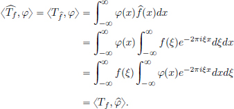
So motivated by this, one could hope to define the Fourier transform of a distribution T by setting

where is the classical Fourier transform of φ ∈ D(R), defined by

But the above calculation is all wrong! Indeed, for a test function φ ∈ D(R), the Fourier transform may not have compact support¹¹, and so does not belong to D(R) (unless φ = 0). In light of this problem (that the Fourier transform of test functions are no longer test functions), it makes sense to work with a bigger class of test functions that are closed under Fourier transformation, and then work with only those distributions that are well-behaved with this larger class of test functions (and then these distributions will be deemed to be “Fourier transform-able”). With this little motivation, we will consider the Schwartz class S(R) of test functions, defined below. Although this story can be developed in R^d with d 1 in general, we will just work with d = 1 here for simplicity.

Definition 6.7. (The Schwartz space S(R) of test functions).

The Schwartz space S(R) of test functions is the set of all functions φ : R → C such that:

(a)φ is infinitely many times differentiable, and

(b)for all nonnegative integers ℓ, m, .

With pointwise operations, S(R) is a vector space.

S(R) is closed under differentiation, and multiplication by polynomials.

It is also immediate that D(R) ⊂ S(R).

An example of a function in S(R)\D(R) is e^−x2.

Exercise 6.25. Show that e^−x2 ∈ S(R).

Definition 6.8. (Convergence in S(R)).

A sequence (φ_n)_n is said to converge to 0 in S(R), written , if for all nonnegative integers ℓ, m, we have .

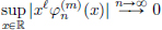Exercise 6.26.

Show that if (φ_n)_n∈N is a sequence of test functions in D(R) such that , then we have

The following result can be shown, but it will take us a bit far afield, and so we skip its somewhat technical proof.

Proposition 6.4.

: S(R) → S(R) is a (linear and) continuous map, that is,

(1)If φ ∈ S(R), then ∈ S(R).

(2)If (φ_n)_n∈N is a sequence in S(R) such that as n → ∞, then .

Definition 6.9. (Tempered distribution).

A tempered distribution T on R is a map T : S(R) → C such that

(1)T is linear, and

(2)if (φ_n)_n∈N is a sequence in S(R) such that as n → ∞, then 〈T, φ_n〉 → 0.

The vector space of all tempered distributions (with pointwise operations) is denoted by S′(R).

Also, since D(R) ⊂ S(R), and since the inclusion is continuous in the sense of Exercise 6.26, it follows that S′(R)⊂ D′(R).

However, it can be shown that the inclusion S′(R) ⊂ D′(R) is strict, as shown below:

Example 6.13. (e^x2 ∈ D′(R)\S′(R)).

e^x2, being continuous, is locally integrable, and hence T_e^x2 ∈ D′(R).

But e^x2 does not define a tempered distribution, since, for example, its action on the test function e^−x2 ∈ S(R), is not finite:

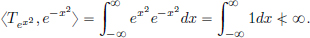
Thus T_e^x2 ∉ S′(R).

Example 6.14. (L¹(R) ⊂ S′(R)).

Let f ∈ L¹, that is, ||f||₁ := |f(x)|dx < ∞.

We claim that the regular distribution T_f is tempered, that is, T ∈ S′(R).

For φ ∈ S(R), |〈T_f, φ〉| = f(x)φ(x)dx |f(x)||φ(x)|dx ||f||₁||φ||_∞.

From here it follows that if (φ_n)_n∈N is a sequence in S(R) such that as n → ∞, then 〈T, φ_n〉 → 0. Hence T_f ∈ S′(R).

Example 6.15. (δ ∈ S′(R)).

The map : S(R) → C is clearly linear.

It is also continuous, since if , then, in particular, φ_n(0) → 0.

Exercise 6.27. (L^∞(R) ⊂ S′(R)).

Show that if f is a bounded function on R, then T_f ∈ S′(R).

Derivative of tempered distributions.

If T ∈ S′(R), then we define T′ : S′(R) → C by

It is easy to see that T′ ∈ S′(R).

Multiplication of tempered distributions by polynomials.

Recall that elements of D′(R) could be multiplied by C^∞ functions. This luxury is not available for tempered distributions: just think of multiplying the constant function 1 ∈ L^∞(R) ⊂ S′(R) by e^x2 ∈ C^∞(R): their product is not tempered, since by Example 6.13, we know that e^x2 ∉ S′(R)!

But while elements in S′(R) can’t be multiplied by general α ∈ C^∞(R), they can nevertheless be multiplied with polynomials as follows:

For T ∈ S′(R), we define xT : S(R) → C by

Then it is easy to see that xT ∈ S′(R).

Fourier transformation of tempered distributions.

Definition 6.10. (Fourier transform of tempered distributions).

If T ∈ S′(R), then its Fourier transform is the tempered distribution

, defined by 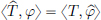, for all φ ∈ S(R).

Using Proposition 6.4, we can see that : S(R) → C defines a tempered distribution.

Exercise 6.28. Show that if f ∈ L¹(R), then .

Example 6.16. (Fourier transform of the Dirac δ).
For φ ∈ S(R), we have that

So the Fourier transform of the tempered distribution δ is the regular tempered distribution corresponding to the constant function 1.

Much of the classical Fourier transform theory, can be extended appropriately for the class of tempered distributions. For example, for tempered distributions T ∈ S′(R), we have

This plays an important role in linear differential equation theory: by taking Fourier transforms, the analytic operation of differentiation is converted into the algebraic operation of multiplication by the Fourier transform variable. Another instance is “convolution theorem”: we know that if f, g ∈ L¹(R), then multiplication on the Fourier transform side corresponds to convolution:

Under certain technical conditions12 on distributions T, S ∈ D′(R), one can define their convolution T ∗ S ∈ D′(R). Then a distributional analogue of the convolution theorem is often available: for example, for T ∈ S′(R), and for a “compactly supported” S ∈ D′(R), one has¹³

These results allow one to rigorously justify some of the formal calculations met in engineering. It also gives rise to some important auxiliary concepts, useful in the theory of PDEs. One such notion, related to convolution of distributions, is the concept of a fundamental solution for a linear PDE.

Definition 6.11. (Fundamental Solution).

Given a linear partial differential operator with constant coefficients,

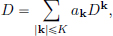
a fundamental solution is a distribution E ∈ D′(R^d) such that

In the above, for a multi-index k = (k₁, · · · , k_d), |k| := k₁ + · · · + k_d.

Fundamental solutions are useful, since they allow one to solve the inhomogeneous equation

For suitable g, it can be shown that u := E ∗ g does the job:

There is also a deep result¹⁴ saying that every nonzero operator D with constant coefficients has a fundamental solution in D′(R^d). Fundamental solutions with appropriate boundary conditions specific to a PDE problem are sometimes referred to as Green’s functions.

Example 6.17. It follows from Exercise 6.8, page 241, that a fundamental solution for the one-dimensional Laplacian operator

is E_p := |x|/2. In fact if we add to E_p any solution to the homogeneous equation u″ = 0, then it will also be a fundamental solution. So the functions ax + b + |x|/2, with arbitrary constants a and b, are all fundamental solutions of the one-dimensional Laplacian operator.

Notes

Some parts of this chapter are inspired by the lectures on Distribution Theory given by Professor Erik G.F. Thomas at the University of Groningen [Thomas (1996)].

1Although the classical Fourier transform does not exist, it can be shown that in the sense of distributions, the Fourier transform of the constant function 1 is the Dirac delta distribution δ.

²That is, vector spaces with a topology making the vector space operations of addition and scalar multiplication continuous. Normed- and inner product-spaces are particular examples of topological vector spaces, where the topology is given by a norm, but it turns out that there are weaker ways of specifying a topology, which aren’t generated by a norm.

³There were, however, earlier usages of such an object; for example an infinitely tall, unit impulse function was used by Cauchy in the early 19th century. The Dirac delta function as such was introduced as a “convenient notation” by the English physicist Paul Dirac in his book, The Principles of Quantum Mechanics, where he called it the “delta function”, as a continuous analogue of the discrete Kronecker delta.

⁴That is, for every > 0, there exists an N ∈ N such that for all n > N and all x ∈ K, |φ_n(x) − φ(x)| < .

⁵Named after Oliver Heaviside (1850–1925), self-taught English physicist, who among other things, developed an “operational calculus” to solve linear differential equations. His methods were not rigorous, and he faced criticism from mathematicians. The Heaviside operational calculus can be justified using distribution theory; see for example [Schwartz (1966), pages 128–130].

⁶See for example [Pinchover and Rubinstein (2005), page 8].

⁷A motivation for this particular change of variables comes from hindsight, see equation (6.3) on page 246: the aim is to view the integrand in (6.2) as a derivative in one of the variables so that one can apply the fundamental theorem of calculus.

⁸A module is just like a vector space, except that the underlying field is replaced by a ring. For the module D′(R^d) we consider, the underlying ring is C^∞(R^d), with pointwise addition and multiplication. We note that not every nonzero element in C^∞(R^d) has a multiplicative inverse; for example a function which is zero on a strict subset of R^d such as x x₁. This is the only thing which is missing for a ring from the list of satisfied field axioms.

⁹D is hypoelliptic if u ∈ D′ and Du ∈ C^∞ implies u ∈ C^∞.

¹⁰We start with such functions, since we know that for absolutely integrable functions f, the classical Fourier transform is a well-defined function, which is bounded and continuous on R.

¹¹In fact, it can be shown that belongs to D if and only if φ = 0.

¹²See for example, [Hörmander (1990), Chapter IV].

¹³See for example, [Hörmander (1990), Theorem 7.1.15, page 166].

¹⁴Due to Malgrange and Ehrenpreiss.