Chapter 2. A Crash Course in Python
People are still crazy about Python after twenty-five years, which I find hard to believe.
Michael Palin
All new employees at DataSciencester are required to go through new employee orientation, the most interesting part of which is a crash course in Python.
This is not a comprehensive Python tutorial but instead is intended to highlight the parts of the language that will be most important to us (some of which are often not the focus of Python tutorials). If you have never used Python before, you probably want to supplement this with some sort of beginner tutorial.
The Zen of Python
Python has a somewhat Zen description of its design principles, which you can also find inside the Python interpreter itself by typing “import this.”
One of the most discussed of these is:
There should be one—and preferably only one—obvious way to do it.
Code written in accordance with this “obvious” way (which may not be obvious at all to a newcomer) is often described as “Pythonic.” Although this is not a book about Python, we will occasionally contrast Pythonic and non-Pythonic ways of accomplishing the same things, and we will generally favor Pythonic solutions to our problems.
Several others touch on aesthetics:
Beautiful is better than ugly. Explicit is better than implicit. Simple is better than complex.
and represent ideals that we will strive for in our code.
Getting Python
Note
As instructions about how to install things can change, while printed books cannot, up-to-date instructions on how to install Python can be found in the book’s GitHub repo.
If the ones printed here don’t work for you, check those.
You can download Python from Python.org. But if you don’t already have Python, I recommend instead installing the Anaconda distribution, which already includes most of the libraries that you need to do data science.
When I wrote the first version of Data Science from Scratch, Python 2.7 was still the preferred version of most data scientists. Accordingly, the first edition of the book was based on Python 2.7.
In the last several years, however, pretty much everyone who counts has migrated to Python 3. Recent versions of Python have many features that make it easier to write clean code, and we’ll be taking ample advantage of features that are only available in Python 3.6 or later. This means that you should get Python 3.6 or later. (In addition, many useful libraries are ending support for Python 2.7, which is another reason to switch.)
Virtual Environments
Starting in the next chapter, we’ll be using the matplotlib library to generate plots and charts. This library is not a core part of Python; you have to install it yourself. Every data science project you do will require some combination of external libraries, sometimes with specific versions that differ from the specific versions you used for other projects. If you were to have a single Python installation, these libraries would conflict and cause you all sorts of problems.
The standard solution is to use virtual environments, which are sandboxed Python environments that maintain their own versions of Python libraries (and, depending on how you set up the environment, of Python itself).
I recommended you install the Anaconda Python distribution, so in this section I’m going to explain how Anaconda’s environments work.
If you are not using Anaconda, you can either use the built-in
venv module
or install
virtualenv. In which case
you should follow their instructions instead.
To create an (Anaconda) virtual environment, you just do the following:
# create a Python 3.6 environment named "dsfs"conda create -n dsfspython=3.6
Follow the prompts, and you’ll have a virtual environment called “dsfs,” with the instructions:
## To activate this environment, use:# > source activate dsfs## To deactivate an active environment, use:# > source deactivate#
As indicated, you then activate the environment using:
source activate dsfsat which point your command prompt should change to indicate the active environment. On my MacBook the prompt now looks like:
(dsfs)ip-10-0-0-198:~ joelg$
As long as this environment is active, any libraries you install will be installed only in the dsfs environment. Once you finish this book and go on to your own projects, you should create your own environments for them.
Now that you have your environment, it’s worth installing IPython, which is a full-featured Python shell:
python -m pip install ipython
Note
Anaconda comes with its own package manager, conda,
but you can also just use the standard Python package manager pip,
which is what we’ll be doing.
The rest of this book will assume that you have created and activated such a Python 3.6 virtual environment (although you can call it whatever you want), and later chapters may rely on the libraries that I told you to install in earlier chapters.
As a matter of good discipline, you should always work in a virtual environment, and never using the “base” Python installation.
Whitespace Formatting
Many languages use curly braces to delimit blocks of code. Python uses indentation:
# The pound sign marks the start of a comment. Python itself# ignores the comments, but they're helpful for anyone reading the code.foriin[1,2,3,4,5]:(i)# first line in "for i" blockforjin[1,2,3,4,5]:(j)# first line in "for j" block(i+j)# last line in "for j" block(i)# last line in "for i" block("done looping")
This makes Python code very readable, but it also means that you have to be very careful with your formatting.
Warning
Programmers will often argue over whether to use tabs or spaces for indentation. For many languages it doesn’t matter that much; however, Python considers tabs and spaces different indentation and will not be able to run your code if you mix the two. When writing Python you should always use spaces, never tabs. (If you write code in an editor you can configure it so that the Tab key just inserts spaces.)
Whitespace is ignored inside parentheses and brackets, which can be helpful for long-winded computations:
long_winded_computation=(1+2+3+4+5+6+7+8+9+10+11+12+13+14+15+16+17+18+19+20)
and for making code easier to read:
list_of_lists=[[1,2,3],[4,5,6],[7,8,9]]easier_to_read_list_of_lists=[[1,2,3],[4,5,6],[7,8,9]]
You can also use a backslash to indicate that a statement continues onto the next line, although we’ll rarely do this:
two_plus_three=2+\3
One consequence of whitespace formatting is that it can be hard to copy and paste code into the Python shell. For example, if you tried to paste the code:
foriin[1,2,3,4,5]:# notice the blank line(i)
into the ordinary Python shell, you would receive the complaint:
IndentationError: expected an indented block
because the interpreter thinks the blank line signals the end of the for loop’s block.
IPython has a magic function called %paste, which correctly pastes whatever is on your clipboard, whitespace and all. This alone is a good reason to use IPython.
Modules
Certain features of Python are not loaded by default. These include both features that are included as part of the language as well as third-party features that you download yourself. In order to use these features, you’ll need to import the modules that contain them.
One approach is to simply import the module itself:
importremy_regex=re.compile("[0-9]+",re.I)
Here, re is the module containing functions and constants for working with regular expressions. After this type of import you must prefix those functions with re. in order to access them.
If you already had a different re in your code, you could use an alias:
importreasregexmy_regex=regex.compile("[0-9]+",regex.I)
You might also do this if your module has an unwieldy name or if you’re going to be typing it a lot. For example, a standard convention when visualizing data with matplotlib is:
importmatplotlib.pyplotaspltplt.plot(...)
If you need a few specific values from a module, you can import them explicitly and use them without qualification:
fromcollectionsimportdefaultdict,Counterlookup=defaultdict(int)my_counter=Counter()
If you were a bad person, you could import the entire contents of a module into your namespace, which might inadvertently overwrite variables you’ve already defined:
match=10fromreimport*# uh oh, re has a match function(match)# "<function match at 0x10281e6a8>"
However, since you are not a bad person, you won’t ever do this.
Functions
A function is a rule for taking zero or more inputs and returning a corresponding output. In Python, we typically define functions using def:
defdouble(x):"""This is where you put an optional docstring that explains what thefunction does. For example, this function multiplies its input by 2."""returnx*2
Python functions are first-class, which means that we can assign them to variables and pass them into functions just like any other arguments:
defapply_to_one(f):"""Calls the function f with 1 as its argument"""returnf(1)my_double=double# refers to the previously defined functionx=apply_to_one(my_double)# equals 2
It is also easy to create short anonymous functions, or lambdas:
y=apply_to_one(lambdax:x+4)# equals 5
You can assign lambdas to variables, although most people will tell you that you should just use def instead:
another_double=lambdax:2*x# don't do thisdefanother_double(x):"""Do this instead"""return2*x
Function parameters can also be given default arguments, which only need to be specified when you want a value other than the default:
defmy_print(message="my default message"):(message)my_print("hello")# prints 'hello'my_print()# prints 'my default message'
It is sometimes useful to specify arguments by name:
deffull_name(first="What's-his-name",last="Something"):returnfirst+" "+lastfull_name("Joel","Grus")# "Joel Grus"full_name("Joel")# "Joel Something"full_name(last="Grus")# "What's-his-name Grus"
We will be creating many, many functions.
Strings
Strings can be delimited by single or double quotation marks (but the quotes have to match):
single_quoted_string='data science'double_quoted_string="data science"
Python uses backslashes to encode special characters. For example:
tab_string="\t"# represents the tab characterlen(tab_string)# is 1
If you want backslashes as backslashes (which you might in Windows directory names or in regular expressions), you can create raw strings using r"":
not_tab_string=r"\t"# represents the characters '\' and 't'len(not_tab_string)# is 2
You can create multiline strings using three double quotes:
multi_line_string="""This is the first line.and this is the second lineand this is the third line"""
A new feature in Python 3.6 is the f-string, which provides a simple way to substitute values into strings. For example, if we had the first name and last name given separately:
first_name="Joel"last_name="Grus"
we might want to combine them into a full name.
There are multiple ways to construct such a full_name string:
full_name1=first_name+" "+last_name# string additionfull_name2="{0} {1}".format(first_name,last_name)# string.format
but the f-string way is much less unwieldy:
full_name3=f"{first_name} {last_name}"
and we’ll prefer it throughout the book.
Exceptions
When something goes wrong, Python raises an exception. Unhandled, exceptions will cause your program to crash. You can handle them using try and except:
try:(0/0)exceptZeroDivisionError:("cannot divide by zero")
Although in many languages exceptions are considered bad, in Python there is no shame in using them to make your code cleaner, and we will sometimes do so.
Lists
Probably the most fundamental data structure in Python is the list, which is simply an ordered collection (it is similar to what in other languages might be called an array, but with some added functionality):
integer_list=[1,2,3]heterogeneous_list=["string",0.1,True]list_of_lists=[integer_list,heterogeneous_list,[]]list_length=len(integer_list)# equals 3list_sum=sum(integer_list)# equals 6
You can get or set the nth element of a list with square brackets:
x=[0,1,2,3,4,5,6,7,8,9]zero=x[0]# equals 0, lists are 0-indexedone=x[1]# equals 1nine=x[-1]# equals 9, 'Pythonic' for last elementeight=x[-2]# equals 8, 'Pythonic' for next-to-last elementx[0]=-1# now x is [-1, 1, 2, 3, ..., 9]
You can also use square brackets to slice lists. The slice i:j
means all elements from i (inclusive) to j (not inclusive).
If you leave off the start of the slice, you’ll slice from the beginning
of the list, and if you leave of the end of the slice, you’ll slice until the
end of the list:
first_three=x[:3]# [-1, 1, 2]three_to_end=x[3:]# [3, 4, ..., 9]one_to_four=x[1:5]# [1, 2, 3, 4]last_three=x[-3:]# [7, 8, 9]without_first_and_last=x[1:-1]# [1, 2, ..., 8]copy_of_x=x[:]# [-1, 1, 2, ..., 9]
You can similarly slice strings and other “sequential” types.
A slice can take a third argument to indicate its stride, which can be negative:
every_third=x[::3]# [-1, 3, 6, 9]five_to_three=x[5:2:-1]# [5, 4, 3]
Python has an in operator to check for list membership:
1in[1,2,3]# True0in[1,2,3]# False
This check involves examining the elements of the list one at a time, which means that you probably shouldn’t use it unless you know your list is pretty small (or unless you don’t care how long the check takes).
It is easy to concatenate lists together. If you want to modify a list in place,
you can use extend to add items from another collection:
x=[1,2,3]x.extend([4,5,6])# x is now [1, 2, 3, 4, 5, 6]
If you don’t want to modify x, you can use list addition:
x=[1,2,3]y=x+[4,5,6]# y is [1, 2, 3, 4, 5, 6]; x is unchanged
More frequently we will append to lists one item at a time:
x=[1,2,3]x.append(0)# x is now [1, 2, 3, 0]y=x[-1]# equals 0z=len(x)# equals 4
It’s often convenient to unpack lists when you know how many elements they contain:
x,y=[1,2]# now x is 1, y is 2
although you will get a ValueError if you don’t have the same number of elements on both sides.
A common idiom is to use an underscore for a value you’re going to throw away:
_,y=[1,2]# now y == 2, didn't care about the first element
Tuples
Tuples are lists’ immutable cousins. Pretty much anything you can do to a list that doesn’t involve modifying it, you can do to a tuple. You specify a tuple by using parentheses (or nothing) instead of square brackets:
my_list=[1,2]my_tuple=(1,2)other_tuple=3,4my_list[1]=3# my_list is now [1, 3]try:my_tuple[1]=3exceptTypeError:("cannot modify a tuple")
Tuples are a convenient way to return multiple values from functions:
defsum_and_product(x,y):return(x+y),(x*y)sp=sum_and_product(2,3)# sp is (5, 6)s,p=sum_and_product(5,10)# s is 15, p is 50
Tuples (and lists) can also be used for multiple assignment:
x,y=1,2# now x is 1, y is 2x,y=y,x# Pythonic way to swap variables; now x is 2, y is 1
Dictionaries
Another fundamental data structure is a dictionary, which associates values with keys and allows you to quickly retrieve the value corresponding to a given key:
empty_dict={}# Pythonicempty_dict2=dict()# less Pythonicgrades={"Joel":80,"Tim":95}# dictionary literal
You can look up the value for a key using square brackets:
joels_grade=grades["Joel"]# equals 80
But you’ll get a KeyError if you ask for a key that’s not in the dictionary:
try:kates_grade=grades["Kate"]exceptKeyError:("no grade for Kate!")
You can check for the existence of a key using in:
joel_has_grade="Joel"ingrades# Truekate_has_grade="Kate"ingrades# False
This membership check is fast even for large dictionaries.
Dictionaries have a get method that returns a default value (instead of raising an exception) when you look up a key that’s not in the dictionary:
joels_grade=grades.get("Joel",0)# equals 80kates_grade=grades.get("Kate",0)# equals 0no_ones_grade=grades.get("No One")# default is None
You can assign key/value pairs using the same square brackets:
grades["Tim"]=99# replaces the old valuegrades["Kate"]=100# adds a third entrynum_students=len(grades)# equals 3
As you saw in Chapter 1, you can use dictionaries to represent structured data:
tweet={"user":"joelgrus","text":"Data Science is Awesome","retweet_count":100,"hashtags":["#data","#science","#datascience","#awesome","#yolo"]}
although we’ll soon see a better approach.
Besides looking for specific keys, we can look at all of them:
tweet_keys=tweet.keys()# iterable for the keystweet_values=tweet.values()# iterable for the valuestweet_items=tweet.items()# iterable for the (key, value) tuples"user"intweet_keys# True, but not Pythonic"user"intweet# Pythonic way of checking for keys"joelgrus"intweet_values# True (slow but the only way to check)
Dictionary keys must be “hashable”; in particular, you cannot use lists as keys. If you need a multipart key, you should probably use a tuple or figure out a way to turn the key into a string.
defaultdict
Imagine that you’re trying to count the words in a document. An obvious approach is to create a dictionary in which the keys are words and the values are counts. As you check each word, you can increment its count if it’s already in the dictionary and add it to the dictionary if it’s not:
word_counts={}forwordindocument:ifwordinword_counts:word_counts[word]+=1else:word_counts[word]=1
You could also use the “forgiveness is better than permission” approach and just handle the exception from trying to look up a missing key:
word_counts={}forwordindocument:try:word_counts[word]+=1exceptKeyError:word_counts[word]=1
A third approach is to use get, which behaves gracefully for missing keys:
word_counts={}forwordindocument:previous_count=word_counts.get(word,0)word_counts[word]=previous_count+1
Every one of these is slightly unwieldy, which is why defaultdict is useful. A defaultdict is like a regular dictionary, except that when you try to look up a key it doesn’t contain, it first adds a value for it using a zero-argument function you provided when you created it. In order to use defaultdicts, you have to import them from collections:
fromcollectionsimportdefaultdictword_counts=defaultdict(int)# int() produces 0forwordindocument:word_counts[word]+=1
They can also be useful with list or dict, or even your own functions:
dd_list=defaultdict(list)# list() produces an empty listdd_list[2].append(1)# now dd_list contains {2: [1]}dd_dict=defaultdict(dict)# dict() produces an empty dictdd_dict["Joel"]["City"]="Seattle"# {"Joel" : {"City": Seattle"}}dd_pair=defaultdict(lambda:[0,0])dd_pair[2][1]=1# now dd_pair contains {2: [0, 1]}
These will be useful when we’re using dictionaries to “collect” results by some key and don’t want to have to check every time to see if the key exists yet.
Counters
A Counter turns a sequence of values into a defaultdict(int)-like object mapping keys to counts:
fromcollectionsimportCounterc=Counter([0,1,2,0])# c is (basically) {0: 2, 1: 1, 2: 1}
This gives us a very simple way to solve our word_counts problem:
# recall, document is a list of wordsword_counts=Counter(document)
A Counter instance has a most_common method that is frequently useful:
# print the 10 most common words and their countsforword,countinword_counts.most_common(10):(word,count)
Sets
Another useful data structure is set, which represents a collection of distinct elements. You can define a set by listing its elements between curly braces:
primes_below_10={2,3,5,7}
However, that doesn’t work for empty sets, as {} already means “empty dict.” In that case you’ll need to use set() itself:
s=set()s.add(1)# s is now {1}s.add(2)# s is now {1, 2}s.add(2)# s is still {1, 2}x=len(s)# equals 2y=2ins# equals Truez=3ins# equals False
We’ll use sets for two main reasons. The first is that in is a very fast operation on sets. If we have a large collection of items that we want to use for a membership test, a set is more appropriate than a list:
stopwords_list=["a","an","at"]+hundreds_of_other_words+["yet","you"]"zip"instopwords_list# False, but have to check every elementstopwords_set=set(stopwords_list)"zip"instopwords_set# very fast to check
The second reason is to find the distinct items in a collection:
item_list=[1,2,3,1,2,3]num_items=len(item_list)# 6item_set=set(item_list)# {1, 2, 3}num_distinct_items=len(item_set)# 3distinct_item_list=list(item_set)# [1, 2, 3]
We’ll use sets less frequently than dictionaries and lists.
Control Flow
As in most programming languages, you can perform an action conditionally using if:
if1>2:message="if only 1 were greater than two..."elif1>3:message="elif stands for 'else if'"else:message="when all else fails use else (if you want to)"
You can also write a ternary if-then-else on one line, which we will do occasionally:
parity="even"ifx%2==0else"odd"
x=0whilex<10:(f"{x} is less than 10")x+=1
although more often we’ll use for and in:
# range(10) is the numbers 0, 1, ..., 9forxinrange(10):(f"{x} is less than 10")
If you need more complex logic, you can use continue and break:
forxinrange(10):ifx==3:continue# go immediately to the next iterationifx==5:break# quit the loop entirely(x)
This will print 0, 1, 2, and 4.
Truthiness
Booleans in Python work as in most other languages, except that they’re capitalized:
one_is_less_than_two=1<2# equals Truetrue_equals_false=True==False# equals False
Python uses the value None to indicate a nonexistent value. It is similar to other languages’ null:
x=Noneassertx==None,"this is the not the Pythonic way to check for None"assertxisNone,"this is the Pythonic way to check for None"
Python lets you use any value where it expects a Boolean. The following are all “falsy”:
-
False -
None -
[](an emptylist) -
{}(an emptydict) -
"" -
set() -
0 -
0.0
Pretty much anything else gets treated as True. This allows you to easily use if statements to test for empty lists, empty strings, empty dictionaries, and so on. It also sometimes causes tricky bugs if you’re not expecting this behavior:
s=some_function_that_returns_a_string()ifs:first_char=s[0]else:first_char=""
A shorter (but possibly more confusing) way of doing the same is:
first_char=sands[0]
since and returns its second value when the first is “truthy,” and the first value when it’s not. Similarly, if x is either a number or possibly None:
safe_x=xor0
is definitely a number, although:
safe_x=xifxisnotNoneelse0
is possibly more readable.
Python has an all function, which takes an iterable and returns True precisely when every element is truthy, and an any function, which returns True when at least one element is truthy:
all([True,1,{3}])# True, all are truthyall([True,1,{}])# False, {} is falsyany([True,1,{}])# True, True is truthyall([])# True, no falsy elements in the listany([])# False, no truthy elements in the list
Sorting
Every Python list has a sort method that sorts it in place. If you don’t want to mess up your list, you can use the sorted function, which returns a new list:
x=[4,1,2,3]y=sorted(x)# y is [1, 2, 3, 4], x is unchangedx.sort()# now x is [1, 2, 3, 4]
By default, sort (and sorted) sort a list from smallest to largest based on naively comparing the elements to one another.
If you want elements sorted from largest to smallest, you can specify a reverse=True parameter. And instead of comparing the elements themselves, you can compare the results of a function that you specify with key:
# sort the list by absolute value from largest to smallestx=sorted([-4,1,-2,3],key=abs,reverse=True)# is [-4, 3, -2, 1]# sort the words and counts from highest count to lowestwc=sorted(word_counts.items(),key=lambdaword_and_count:word_and_count[1],reverse=True)
List Comprehensions
Frequently, you’ll want to transform a list into another list by choosing only certain elements, by transforming elements, or both. The Pythonic way to do this is with list comprehensions:
even_numbers=[xforxinrange(5)ifx%2==0]# [0, 2, 4]squares=[x*xforxinrange(5)]# [0, 1, 4, 9, 16]even_squares=[x*xforxineven_numbers]# [0, 4, 16]
You can similarly turn lists into dictionaries or sets:
square_dict={x:x*xforxinrange(5)}# {0: 0, 1: 1, 2: 4, 3: 9, 4: 16}square_set={x*xforxin[1,-1]}# {1}
If you don’t need the value from the list, it’s common to use an underscore as the variable:
zeros=[0for_ineven_numbers]# has the same length as even_numbers
A list comprehension can include multiple fors:
pairs=[(x,y)forxinrange(10)foryinrange(10)]# 100 pairs (0,0) (0,1) ... (9,8), (9,9)
and later fors can use the results of earlier ones:
increasing_pairs=[(x,y)# only pairs with x < y,forxinrange(10)# range(lo, hi) equalsforyinrange(x+1,10)]# [lo, lo + 1, ..., hi - 1]
We will use list comprehensions a lot.
Automated Testing and assert
As data scientists, we’ll be writing a lot of code. How can we be confident our code is correct? One way is with types (discussed shortly), but another way is with automated tests.
There are elaborate frameworks for writing and running tests,
but in this book we’ll restrict ourselves to using assert
statements, which will cause your code to raise an AssertionError
if your specified condition is not truthy:
assert1+1==2assert1+1==2,"1 + 1 should equal 2 but didn't"
As you can see in the second case, you can optionally add a message to be printed if the assertion fails.
It’s not particularly interesting to assert that 1 + 1 = 2. What’s more interesting is to assert that functions you write are doing what you expect them to:
defsmallest_item(xs):returnmin(xs)assertsmallest_item([10,20,5,40])==5assertsmallest_item([1,0,-1,2])==-1
Throughout the book we’ll be using assert in this way.
It is a good practice, and I strongly encourage you to make liberal use of it in your own code.
(If you look at the book’s code on GitHub, you will see that it contains many, many
more assert statements than are printed in the book. This helps me be confident that
the code I’ve written for you is correct.)
Another less common use is to assert things about inputs to functions:
defsmallest_item(xs):assertxs,"empty list has no smallest item"returnmin(xs)
We’ll occasionally do this, but more often we’ll use assert to check that our code is correct.
Object-Oriented Programming
Like many languages, Python allows you to define classes that encapsulate data and the functions that operate on them. We’ll use them sometimes to make our code cleaner and simpler. It’s probably simplest to explain them by constructing a heavily annotated example.
Here we’ll construct a class representing a “counting clicker,” the sort that is used at the door to track how many people have shown up for the “advanced topics in data science” meetup.
It maintains a count, can be clicked to increment the count,
allows you to read_count,
and can be reset back to zero.
(In real life one of these rolls over from 9999 to 0000, but we won’t bother with that.)
To define a class, you use the class keyword and a PascalCase name:
classCountingClicker:"""A class can/should have a docstring, just like a function"""
A class contains zero or more member functions.
By convention, each takes a first parameter, self, that refers
to the particular class instance.
Normally, a class has a constructor, named __init__.
It takes whatever parameters you need to construct an instance
of your class and does whatever setup you need:
def__init__(self,count=0):self.count=count
Although the constructor has a funny name, we construct instances of the clicker using just the class name:
clicker1=CountingClicker()# initialized to 0clicker2=CountingClicker(100)# starts with count=100clicker3=CountingClicker(count=100)# more explicit way of doing the same
Notice that the __init__ method name starts and ends with double underscores.
These “magic” methods are sometimes called “dunder” methods (double-UNDERscore, get it?)
and represent “special” behaviors.
Note
Class methods whose names start with an underscore are—by convention—considered “private,” and users of the class are not supposed to directly call them. However, Python will not stop users from calling them.
Another such method is __repr__, which produces
the string representation of a class instance:
def__repr__(self):returnf"CountingClicker(count={self.count})"
And finally we need to implement the public API of our class:
defclick(self,num_times=1):"""Click the clicker some number of times."""self.count+=num_timesdefread(self):returnself.countdefreset(self):self.count=0
Having defined it, let’s use assert to write some test cases for our clicker:
clicker=CountingClicker()assertclicker.read()==0,"clicker should start with count 0"clicker.click()clicker.click()assertclicker.read()==2,"after two clicks, clicker should have count 2"clicker.reset()assertclicker.read()==0,"after reset, clicker should be back to 0"
Writing tests like these help us be confident that our code is working the way it’s designed to, and that it remains doing so whenever we make changes to it.
We’ll also occasionally create subclasses that inherit some of their functionality from a parent class. For example, we could create a non-reset-able clicker by using CountingClicker as the base class and overriding the reset method to do nothing:
# A subclass inherits all the behavior of its parent class.classNoResetClicker(CountingClicker):# This class has all the same methods as CountingClicker# Except that it has a reset method that does nothing.defreset(self):passclicker2=NoResetClicker()assertclicker2.read()==0clicker2.click()assertclicker2.read()==1clicker2.reset()assertclicker2.read()==1,"reset shouldn't do anything"
Iterables and Generators
One nice thing about a list is that you can retrieve specific elements by their indices. But you don’t always need this! A list of a billion numbers takes up a lot of memory. If you only want the elements one at a time, there’s no good reason to keep them all around. If you only end up needing the first several elements, generating the entire billion is hugely wasteful.
Often all we need is to iterate over the collection using for and in.
In this case we can create generators, which
can be iterated over just like lists but generate their values lazily on demand.
One way to create generators is with functions and the yield operator:
defgenerate_range(n):i=0whilei<n:yieldi# every call to yield produces a value of the generatori+=1
The following loop will consume the yielded values one at a time until none are left:
foriingenerate_range(10):(f"i: {i}")
(In fact, range is itself lazy, so there’s no point in doing this.)
With a generator, you can even create an infinite sequence:
defnatural_numbers():"""returns 1, 2, 3, ..."""n=1whileTrue:yieldnn+=1
although you probably shouldn’t iterate over it without using some kind of break logic.
Tip
The flip side of laziness is that you can only iterate through a generator once. If you need to iterate through something multiple times, you’ll need to either re-create the generator each time or use a list. If generating the values is expensive, that might be a good reason to use a list instead.
A second way to create generators is by using for comprehensions wrapped in parentheses:
evens_below_20=(iforiingenerate_range(20)ifi%2==0)
Such a “generator comprehension” doesn’t do any work until
you iterate over it (using for or next). We can use this
to build up elaborate data-processing pipelines:
# None of these computations *does* anything until we iteratedata=natural_numbers()evens=(xforxindataifx%2==0)even_squares=(x**2forxinevens)even_squares_ending_in_six=(xforxineven_squaresifx%10==6)# and so on
Not infrequently, when we’re iterating over a list or a generator
we’ll want not just the values but also their indices. For this common
case Python provides an enumerate function, which turns values
into pairs (index, value):
names=["Alice","Bob","Charlie","Debbie"]# not Pythonicforiinrange(len(names)):(f"name {i} is {names[i]}")# also not Pythonici=0fornameinnames:(f"name {i} is {names[i]}")i+=1# Pythonicfori,nameinenumerate(names):(f"name {i} is {name}")
We’ll use this a lot.
Randomness
As we learn data science, we will frequently need to generate random numbers,
which we can do with the random module:
importrandomrandom.seed(10)# this ensures we get the same results every timefour_uniform_randoms=[random.random()for_inrange(4)]# [0.5714025946899135, # random.random() produces numbers# 0.4288890546751146, # uniformly between 0 and 1.# 0.5780913011344704, # It's the random function we'll use# 0.20609823213950174] # most often.
The random module actually produces pseudorandom (that is, deterministic) numbers
based on an internal state that you can set with random.seed if you want to get
reproducible results:
random.seed(10)# set the seed to 10(random.random())# 0.57140259469random.seed(10)# reset the seed to 10(random.random())# 0.57140259469 again
We’ll sometimes use random.randrange, which takes either one or two arguments and returns an element chosen randomly from the corresponding range:
random.randrange(10)# choose randomly from range(10) = [0, 1, ..., 9]random.randrange(3,6)# choose randomly from range(3, 6) = [3, 4, 5]
There are a few more methods that we’ll sometimes find convenient. For example, random.shuffle randomly reorders the elements of a list:
up_to_ten=[1,2,3,4,5,6,7,8,9,10]random.shuffle(up_to_ten)(up_to_ten)# [7, 2, 6, 8, 9, 4, 10, 1, 3, 5] (your results will probably be different)
If you need to randomly pick one element from a list, you can use random.choice:
my_best_friend=random.choice(["Alice","Bob","Charlie"])# "Bob" for me
And if you need to randomly choose a sample of elements without replacement (i.e., with no duplicates), you can use random.sample:
lottery_numbers=range(60)winning_numbers=random.sample(lottery_numbers,6)# [16, 36, 10, 6, 25, 9]
To choose a sample of elements with replacement (i.e., allowing duplicates), you can just make multiple calls to random.choice:
four_with_replacement=[random.choice(range(10))for_inrange(4)](four_with_replacement)# [9, 4, 4, 2]
Regular Expressions
Regular expressions provide a way of searching text. They are incredibly useful, but also fairly complicated—so much so that there are entire books written about them. We will get into their details the few times we encounter them; here are a few examples of how to use them in Python:
importrere_examples=[# All of these are True, becausenotre.match("a","cat"),# 'cat' doesn't start with 'a're.search("a","cat"),# 'cat' has an 'a' in itnotre.search("c","dog"),# 'dog' doesn't have a 'c' in it.3==len(re.split("[ab]","carbs")),# Split on a or b to ['c','r','s']."R-D-"==re.sub("[0-9]","-","R2D2")# Replace digits with dashes.]assertall(re_examples),"all the regex examples should be True"
One important thing to note is that re.match checks whether the beginning of a string
matches a regular expression, while re.search checks whether any part of a string
matches a regular expression. At some point you will mix these two up and it will cause
you grief.
The official documentation goes into much more detail.
Functional Programming
Note
The first edition of this book introduced the Python functions
partial, map, reduce, and filter at this point. On my journey toward
enlightenment I have realized that these functions are best avoided,
and their uses in the book have been replaced with list comprehensions, for loops, and other, more Pythonic constructs.
zip and Argument Unpacking
Often we will need to zip two or more iterables together. The zip function transforms multiple iterables into a single iterable of tuples of corresponding function:
list1=['a','b','c']list2=[1,2,3]# zip is lazy, so you have to do something like the following[pairforpairinzip(list1,list2)]# is [('a', 1), ('b', 2), ('c', 3)]
If the lists are different lengths, zip stops as soon as the first list ends.
You can also “unzip” a list using a strange trick:
pairs=[('a',1),('b',2),('c',3)]letters,numbers=zip(*pairs)
The asterisk (*) performs argument unpacking, which uses the elements of pairs as individual arguments to zip. It ends up the same as if you’d called:
letters,numbers=zip(('a',1),('b',2),('c',3))
You can use argument unpacking with any function:
defadd(a,b):returna+badd(1,2)# returns 3try:add([1,2])exceptTypeError:("add expects two inputs")add(*[1,2])# returns 3
It is rare that we’ll find this useful, but when we do it’s a neat trick.
args and kwargs
Let’s say we want to create a higher-order function
that takes as input some function f
and returns a new function that for any input returns
twice the value of f:
defdoubler(f):# Here we define a new function that keeps a reference to fdefg(x):return2*f(x)# And return that new functionreturng
This works in some cases:
deff1(x):returnx+1g=doubler(f1)assertg(3)==8,"(3 + 1) * 2 should equal 8"assertg(-1)==0,"(-1 + 1) * 2 should equal 0"
However, it doesn’t work with functions that take more than a single argument:
deff2(x,y):returnx+yg=doubler(f2)try:g(1,2)exceptTypeError:("as defined, g only takes one argument")
What we need is a way to specify a function that takes arbitrary arguments. We can do this with argument unpacking and a little bit of magic:
defmagic(*args,**kwargs):("unnamed args:",args)("keyword args:",kwargs)magic(1,2,key="word",key2="word2")# prints# unnamed args: (1, 2)# keyword args: {'key': 'word', 'key2': 'word2'}
That is, when we define a function like this, args is a tuple of its unnamed arguments
and kwargs is a dict of its named arguments. It works the other way too, if you
want to use a list (or tuple) and dict to supply arguments to a function:
defother_way_magic(x,y,z):returnx+y+zx_y_list=[1,2]z_dict={"z":3}assertother_way_magic(*x_y_list,**z_dict)==6,"1 + 2 + 3 should be 6"
You could do all sorts of strange tricks with this; we will only use it to produce higher-order functions whose inputs can accept arbitrary arguments:
defdoubler_correct(f):"""works no matter what kind of inputs f expects"""defg(*args,**kwargs):"""whatever arguments g is supplied, pass them through to f"""return2*f(*args,**kwargs)returngg=doubler_correct(f2)assertg(1,2)==6,"doubler should work now"
As a general rule, your code will be more correct and more readable
if you are explicit about what sorts of arguments your functions require;
accordingly, we will use args and kwargs only when we have no other option.
Type Annotations
Python is a dynamically typed language. That means that it in general it doesn’t care about the types of objects we use, as long as we use them in valid ways:
defadd(a,b):returna+bassertadd(10,5)==15,"+ is valid for numbers"assertadd([1,2],[3])==[1,2,3],"+ is valid for lists"assertadd("hi ","there")=="hi there","+ is valid for strings"try:add(10,"five")exceptTypeError:("cannot add an int to a string")
whereas in a statically typed language our functions and objects would have specific types:
defadd(a:int,b:int)->int:returna+badd(10,5)# you'd like this to be OKadd("hi ","there")# you'd like this to be not OK
In fact, recent versions of Python do (sort of) have this functionality.
The preceding version of add with the int type annotations is valid Python 3.6!
However, these type annotations don’t actually do anything.
You can still use the annotated add function to add strings,
and the call to add(10, "five") will still raise the exact same TypeError.
That said, there are still (at least) four good reasons to use type annotations in your Python code:
-
Types are an important form of documentation. This is doubly true in a book that is using code to teach you theoretical and mathematical concepts. Compare the following two function stubs:
defdot_product(x,y):...# we have not yet defined Vector, but imagine we haddefdot_product(x:Vector,y:Vector)->float:...I find the second one exceedingly more informative; hopefully you do too. (At this point I have gotten so used to type hinting that I now find untyped Python difficult to read.)
-
There are external tools (the most popular is
mypy) that will read your code, inspect the type annotations, and let you know about type errors before you ever run your code. For example, if you ranmypyover a file containingadd("hi ", "there"), it would warn you:error: Argument 1 to "add" has incompatible type "str"; expected "int"
Like
asserttesting, this is a good way to find mistakes in your code before you ever run it. The narrative in the book will not involve such a type checker; however, behind the scenes I will be running one, which will help ensure that the book itself is correct. -
Having to think about the types in your code forces you to design cleaner functions and interfaces:
fromtypingimportUniondefsecretly_ugly_function(value,operation):...defugly_function(value:int,operation:Union[str,int,float,bool])->int:...Here we have a function whose
operationparameter is allowed to be astring, or anint, or afloat, or abool. It is highly likely that this function is fragile and difficult to use, but it becomes far more clear when the types are made explicit. Doing so, then, will force us to design in a less clunky way, for which our users will thank us. -
Using types allows your editor to help you with things like autocomplete (Figure 2-1) and to get angry at type errors.
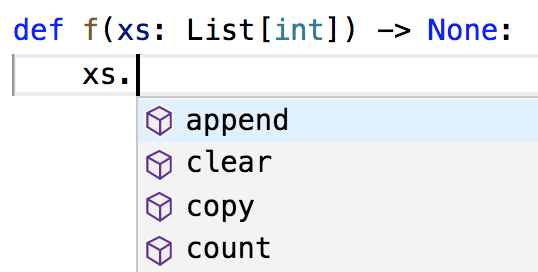
Figure 2-1. VSCode, but likely your editor does the same
Sometimes people insist that type hints may be valuable on large projects but are not worth the time for small ones. However, since type hints take almost no additional time to type and allow your editor to save you time, I maintain that they actually allow you to write code more quickly, even for small projects.
For all these reasons, all of the code in the remainder of the book will use type annotations. I expect that some readers will be put off by the use of type annotations; however, I suspect by the end of the book they will have changed their minds.
How to Write Type Annotations
As we’ve seen, for built-in types like int and bool and float,
you just use the type itself as the annotation. What if you had (say) a list?
deftotal(xs:list)->float:returnsum(total)
This isn’t wrong, but the type is not specific enough.
It’s clear we really want xs to be a list of floats, not (say) a list of strings.
The typing module provides a number of parameterized types that we can use to do just this:
fromtypingimportList# note capital Ldeftotal(xs:List[float])->float:returnsum(total)
Up until now we’ve only specified annotations for function parameters and return types. For variables themselves it’s usually obvious what the type is:
# This is how to type-annotate variables when you define them.# But this is unnecessary; it's "obvious" x is an int.x:int=5
However, sometimes it’s not obvious:
values=[]# what's my type?best_so_far=None# what's my type?
In such cases we will supply inline type hints:
fromtypingimportOptionalvalues:List[int]=[]best_so_far:Optional[float]=None# allowed to be either a float or None
The typing module contains many other types, only a few of which we’ll ever use:
# the type annotations in this snippet are all unnecessaryfromtypingimportDict,Iterable,Tuple# keys are strings, values are intscounts:Dict[str,int]={'data':1,'science':2}# lists and generators are both iterableiflazy:evens:Iterable[int]=(xforxinrange(10)ifx%2==0)else:evens=[0,2,4,6,8]# tuples specify a type for each elementtriple:Tuple[int,float,int]=(10,2.3,5)
Finally, since Python has first-class functions, we need a type to represent those as well. Here’s a pretty contrived example:
fromtypingimportCallable# The type hint says that repeater is a function that takes# two arguments, a string and an int, and returns a string.deftwice(repeater:Callable[[str,int],str],s:str)->str:returnrepeater(s,2)defcomma_repeater(s:str,n:int)->str:n_copies=[sfor_inrange(n)]return', '.join(n_copies)asserttwice(comma_repeater,"type hints")=="type hints, type hints"
As type annotations are just Python objects, we can assign them to variables to make them easier to refer to:
Number=intNumbers=List[Number]deftotal(xs:Numbers)->Number:returnsum(xs)
By the time you get to the end of the book, you’ll be quite familiar with reading and writing type annotations, and I hope you’ll use them in your code.
Welcome to DataSciencester!
This concludes new employee orientation. Oh, and also: try not to embezzle anything.
For Further Exploration
-
There is no shortage of Python tutorials in the world. The official one is not a bad place to start.
-
The official IPython tutorial will help you get started with IPython, if you decide to use it. Please use it.
-
The
mypydocumentation will tell you more than you ever wanted to know about Python type annotations and type checking.