Chapter 10. Working with Data

Experts often possess more data than judgment.

Colin Powell

Working with data is both an art and a science. We’ve mostly been talking about the science part, but in this chapter we’ll look at some of the art.

Exploring Your Data

After you’ve identified the questions you’re trying to answer and have gotten your hands on some data, you might be tempted to dive in and immediately start building models and getting answers. But you should resist this urge. Your first step should be to explore your data.

Exploring One-Dimensional Data

The simplest case is when you have a one-dimensional dataset, which is just a collection of numbers. For example, these could be the daily average number of minutes each user spends on your site, the number of times each of a collection of data science tutorial videos was watched, or the number of pages of each of the data science books in your data science library.

An obvious first step is to compute a few summary statistics. You’d like to know how many data points you have, the smallest, the largest, the mean, and the standard deviation.

But even these don’t necessarily give you a great understanding. A good next step is to create a histogram, in which you group your data into discrete buckets and count how many points fall into each bucket:

from typing import List, Dict
from collections import Counter
import math

import matplotlib.pyplot as plt

def bucketize(point: float, bucket_size: float) -> float:
    """Floor the point to the next lower multiple of bucket_size"""
    return bucket_size * math.floor(point / bucket_size)

def make_histogram(points: List[float], bucket_size: float) -> Dict[float, int]:
    """Buckets the points and counts how many in each bucket"""
    return Counter(bucketize(point, bucket_size) for point in points)

def plot_histogram(points: List[float], bucket_size: float, title: str = ""):
    histogram = make_histogram(points, bucket_size)
    plt.bar(histogram.keys(), histogram.values(), width=bucket_size)
    plt.title(title)

For example, consider the two following sets of data:

import random
from scratch.probability import inverse_normal_cdf

random.seed(0)

# uniform between -100 and 100
uniform = [200 * random.random() - 100 for _ in range(10000)]

# normal distribution with mean 0, standard deviation 57
normal = [57 * inverse_normal_cdf(random.random())
          for _ in range(10000)]

Both have means close to 0 and standard deviations close to 58. However, they have very different distributions. Figure 10-1 shows the distribution of uniform:

plot_histogram(uniform, 10, "Uniform Histogram")

while Figure 10-2 shows the distribution of normal:

plot_histogram(normal, 10, "Normal Histogram")

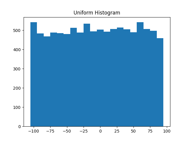
Figure 10-1. Histogram of uniform

In this case the two distributions have a pretty different max and min, but even knowing that wouldn’t have been sufficient to understand how they differed.

Two Dimensions

Now imagine you have a dataset with two dimensions. Maybe in addition to daily minutes you have years of data science experience. Of course you’d want to understand each dimension individually. But you probably also want to scatter the data.

For example, consider another fake dataset:

def random_normal() -> float:
    """Returns a random draw from a standard normal distribution"""
    return inverse_normal_cdf(random.random())

xs = [random_normal() for _ in range(1000)]
ys1 = [ x + random_normal() / 2 for x in xs]
ys2 = [-x + random_normal() / 2 for x in xs]

If you were to run plot_histogram on ys1 and ys2, you’d get similar-looking plots (indeed, both are normally distributed with the same mean and standard deviation).

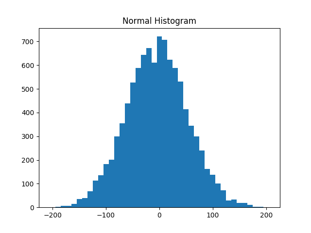
Figure 10-2. Histogram of normal

But each has a very different joint distribution with xs, as shown in Figure 10-3:

plt.scatter(xs, ys1, marker='.', color='black', label='ys1')
plt.scatter(xs, ys2, marker='.', color='gray',  label='ys2')
plt.xlabel('xs')
plt.ylabel('ys')
plt.legend(loc=9)
plt.title("Very Different Joint Distributions")
plt.show()

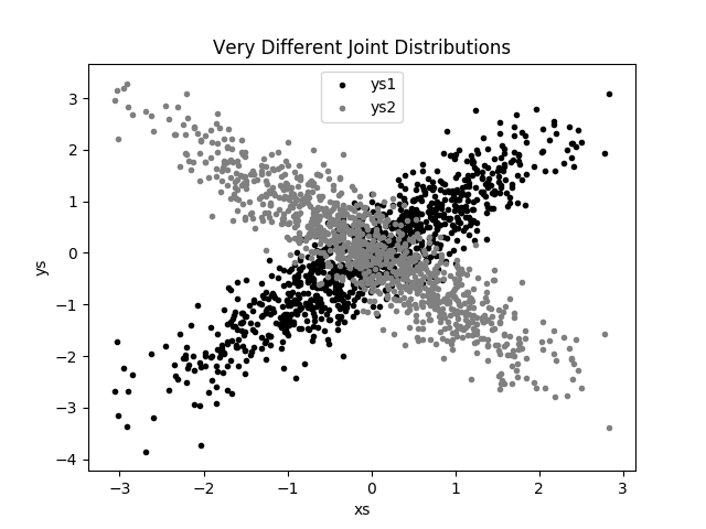
Figure 10-3. Scattering two different ys

This difference would also be apparent if you looked at the correlations:

from scratch.statistics import correlation

print(correlation(xs, ys1))      # about 0.9
print(correlation(xs, ys2))      # about -0.9

Many Dimensions

With many dimensions, you’d like to know how all the dimensions relate to one another. A simple approach is to look at the correlation matrix, in which the entry in row i and column j is the correlation between the ith dimension and the jth dimension of the data:

from scratch.linear_algebra import Matrix, Vector, make_matrix

def correlation_matrix(data: List[Vector]) -> Matrix:
    """
    Returns the len(data) x len(data) matrix whose (i, j)-th entry
    is the correlation between data[i] and data[j]
    """
    def correlation_ij(i: int, j: int) -> float:
        return correlation(data[i], data[j])

    return make_matrix(len(data), len(data), correlation_ij)

A more visual approach (if you don’t have too many dimensions) is to make a scatterplot matrix (Figure 10-4) showing all the pairwise scatterplots. To do that we’ll use plt.subplots, which allows us to create subplots of our chart. We give it the number of rows and the number of columns, and it returns a figure object (which we won’t use) and a two-dimensional array of axes objects (each of which we’ll plot to):

# corr_data is a list of four 100-d vectors
num_vectors = len(corr_data)
fig, ax = plt.subplots(num_vectors, num_vectors)

for i in range(num_vectors):
    for j in range(num_vectors):

        # Scatter column_j on the x-axis vs. column_i on the y-axis
        if i != j: ax[i][j].scatter(corr_data[j], corr_data[i])

        # unless i == j, in which case show the series name
        else: ax[i][j].annotate("series " + str(i), (0.5, 0.5),
                                xycoords='axes fraction',
                                ha="center", va="center")

        # Then hide axis labels except left and bottom charts
        if i < num_vectors - 1: ax[i][j].xaxis.set_visible(False)
        if j > 0: ax[i][j].yaxis.set_visible(False)

# Fix the bottom-right and top-left axis labels, which are wrong because
# their charts only have text in them
ax[-1][-1].set_xlim(ax[0][-1].get_xlim())
ax[0][0].set_ylim(ax[0][1].get_ylim())

plt.show()

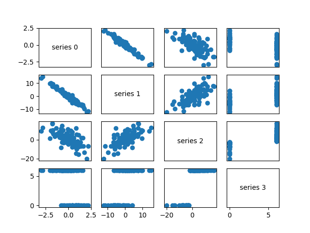
Figure 10-4. Scatterplot matrix

Looking at the scatterplots, you can see that series 1 is very negatively correlated with series 0, series 2 is positively correlated with series 1, and series 3 only takes on the values 0 and 6, with 0 corresponding to small values of series 2 and 6 corresponding to large values.

This is a quick way to get a rough sense of which of your variables are correlated (unless you spend hours tweaking matplotlib to display things exactly the way you want them to, in which case it’s not a quick way).

Using NamedTuples

One common way of representing data is using dicts:

import datetime

stock_price = {'closing_price': 102.06,
               'date': datetime.date(2014, 8, 29),
               'symbol': 'AAPL'}

There are several reasons why this is less than ideal, however. This is a slightly inefficient representation (a dict involves some overhead), so that if you have a lot of stock prices they’ll take up more memory than they have to. For the most part, this is a minor consideration.

A larger issue is that accessing things by dict key is error-prone. The following code will run without error and just do the wrong thing:

# oops, typo
stock_price['cosing_price'] = 103.06

Finally, while we can type-annotate uniform dictionaries:

prices: Dict[datetime.date, float] = {}

there’s no helpful way to annotate dictionaries-as-data that have lots of different value types. So we also lose the power of type hints.

As an alternative, Python includes a namedtuple class, which is like a tuple but with named slots:

from collections import namedtuple

StockPrice = namedtuple('StockPrice', ['symbol', 'date', 'closing_price'])
price = StockPrice('MSFT', datetime.date(2018, 12, 14), 106.03)

assert price.symbol == 'MSFT'
assert price.closing_price == 106.03

Like regular tuples, namedtuples are immutable, which means that you can’t modify their values once they’re created. Occasionally this will get in our way, but mostly that’s a good thing.

You’ll notice that we still haven’t solved the type annotation issue. We do that by using the typed variant, NamedTuple:

from typing import NamedTuple

class StockPrice(NamedTuple):
    symbol: str
    date: datetime.date
    closing_price: float

    def is_high_tech(self) -> bool:
        """It's a class, so we can add methods too"""
        return self.symbol in ['MSFT', 'GOOG', 'FB', 'AMZN', 'AAPL']

price = StockPrice('MSFT', datetime.date(2018, 12, 14), 106.03)

assert price.symbol == 'MSFT'
assert price.closing_price == 106.03
assert price.is_high_tech()

And now your editor can help you out, as shown in Figure 10-5.

Figure 10-5. Helpful editor

Note

Very few people use NamedTuple in this way. But they should!

Dataclasses

Dataclasses are (sort of) a mutable version of NamedTuple. (I say “sort of” because NamedTuples represent their data compactly as tuples, whereas dataclasses are regular Python classes that simply generate some methods for you automatically.)

Note

Dataclasses are new in Python 3.7. If you’re using an older version, this section won’t work for you.

The syntax is very similar to NamedTuple. But instead of inheriting from a base class, we use a decorator:

from dataclasses import dataclass

@dataclass
class StockPrice2:
    symbol: str
    date: datetime.date
    closing_price: float

    def is_high_tech(self) -> bool:
        """It's a class, so we can add methods too"""
        return self.symbol in ['MSFT', 'GOOG', 'FB', 'AMZN', 'AAPL']

price2 = StockPrice2('MSFT', datetime.date(2018, 12, 14), 106.03)

assert price2.symbol == 'MSFT'
assert price2.closing_price == 106.03
assert price2.is_high_tech()

As mentioned, the big difference is that we can modify a dataclass instance’s values:

# stock split
price2.closing_price /= 2
assert price2.closing_price == 51.03

If we tried to modify a field of the NamedTuple version, we’d get an AttributeError.

This also leaves us susceptible to the kind of errors we were hoping to avoid by not using dicts:

# It's a regular class, so add new fields however you like!
price2.cosing_price = 75  # oops

We won’t be using dataclasses, but you may encounter them out in the wild.

Cleaning and Munging

Real-world data is dirty. Often you’ll have to do some work on it before you can use it. We saw examples of this in Chapter 9. We have to convert strings to floats or ints before we can use them. We have to check for missing values and outliers and bad data.

Previously, we did that right before using the data:

closing_price = float(row[2])

But it’s probably less error-prone to do the parsing in a function that we can test:

from dateutil.parser import parse

def parse_row(row: List[str]) -> StockPrice:
    symbol, date, closing_price = row
    return StockPrice(symbol=symbol,
                      date=parse(date).date(),
                      closing_price=float(closing_price))

# Now test our function
stock = parse_row(["MSFT", "2018-12-14", "106.03"])

assert stock.symbol == "MSFT"
assert stock.date == datetime.date(2018, 12, 14)
assert stock.closing_price == 106.03

What if there’s bad data? A “float” value that doesn’t actually represent a number? Maybe you’d rather get a None than crash your program?

from typing import Optional
import re

def try_parse_row(row: List[str]) -> Optional[StockPrice]:
    symbol, date_, closing_price_ = row

    # Stock symbol should be all capital letters
    if not re.match(r"^[A-Z]+$", symbol):
        return None

    try:
        date = parse(date_).date()
    except ValueError:
        return None

    try:
        closing_price = float(closing_price_)
    except ValueError:
        return None

    return StockPrice(symbol, date, closing_price)

# Should return None for errors
assert try_parse_row(["MSFT0", "2018-12-14", "106.03"]) is None
assert try_parse_row(["MSFT", "2018-12--14", "106.03"]) is None
assert try_parse_row(["MSFT", "2018-12-14", "x"]) is None

# But should return same as before if data is good
assert try_parse_row(["MSFT", "2018-12-14", "106.03"]) == stock

For example, if we have comma-delimited stock prices with bad data:

AAPL,6/20/2014,90.91
MSFT,6/20/2014,41.68
FB,6/20/3014,64.5
AAPL,6/19/2014,91.86
MSFT,6/19/2014,n/a
FB,6/19/2014,64.34

we can now read and return only the valid rows:

import csv

data: List[StockPrice] = []

with open("comma_delimited_stock_prices.csv") as f:
    reader = csv.reader(f)
    for row in reader:
        maybe_stock = try_parse_row(row)
        if maybe_stock is None:
            print(f"skipping invalid row: {row}")
        else:
            data.append(maybe_stock)

and decide what we want to do about the invalid ones. Generally speaking, the three options are to get rid of them, to go back to the source and try to fix the bad/missing data, or to do nothing and cross our fingers. If there’s one bad row out of millions, it’s probably okay to ignore it. But if half your rows have bad data, that’s something you need to fix.

A good next step is to check for outliers, using techniques from “Exploring Your Data” or by ad hoc investigating. For example, did you notice that one of the dates in the stocks file had the year 3014? That won’t (necessarily) give you an error, but it’s quite plainly wrong, and you’ll get screwy results if you don’t catch it. Real-world datasets have missing decimal points, extra zeros, typographical errors, and countless other problems that it’s your job to catch. (Maybe it’s not officially your job, but who else is going to do it?)

Manipulating Data

One of the most important skills of a data scientist is manipulating data. It’s more of a general approach than a specific technique, so we’ll just work through a handful of examples to give you the flavor of it.

Imagine we have a bunch of stock price data that looks like this:

data = [
    StockPrice(symbol='MSFT',
               date=datetime.date(2018, 12, 24),
               closing_price=106.03),
    # ...
]

Let’s start asking questions about this data. Along the way we’ll try to notice patterns in what we’re doing and abstract out some tools to make the manipulation easier.

For instance, suppose we want to know the highest-ever closing price for AAPL. Let’s break this down into concrete steps:

1. Restrict ourselves to AAPL rows.

2. Grab the closing_price from each row.

3. Take the max of those prices.

We can do all three at once using a comprehension:

max_aapl_price = max(stock_price.closing_price
                     for stock_price in data
                     if stock_price.symbol == "AAPL")

More generally, we might want to know the highest-ever closing price for each stock in our dataset. One way to do this is:

1. Create a dict to keep track of highest prices (we’ll use a defaultdict that returns minus infinity for missing values, since any price will be greater than that).

2. Iterate over our data, updating it.

Here’s the code:

from collections import defaultdict

max_prices: Dict[str, float] = defaultdict(lambda: float('-inf'))

for sp in data:
    symbol, closing_price = sp.symbol, sp.closing_price
    if closing_price > max_prices[symbol]:
        max_prices[symbol] = closing_price

We can now start to ask more complicated things, like what are the largest and smallest one-day percent changes in our dataset. The percent change is price_today / price_yesterday - 1, which means we need some way of associating today’s price and yesterday’s price. One approach is to group the prices by symbol, and then, within each group:

1. Order the prices by date.

2. Use zip to get (previous, current) pairs.

3. Turn the pairs into new “percent change” rows.

Let’s start by grouping the prices by symbol:

from typing import List
from collections import defaultdict

# Collect the prices by symbol
prices: Dict[str, List[StockPrice]] = defaultdict(list)

for sp in data:
    prices[sp.symbol].append(sp)

Since the prices are tuples, they’ll get sorted by their fields in order: first by symbol, then by date, then by price. This means that if we have some prices all with the same symbol, sort will sort them by date (and then by price, which does nothing, since we only have one per date), which is what we want.

# Order the prices by date
prices = {symbol: sorted(symbol_prices)
          for symbol, symbol_prices in prices.items()}

which we can use to compute a sequence of day-over-day changes:

def pct_change(yesterday: StockPrice, today: StockPrice) -> float:
    return today.closing_price / yesterday.closing_price - 1

class DailyChange(NamedTuple):
    symbol: str
    date: datetime.date
    pct_change: float

def day_over_day_changes(prices: List[StockPrice]) -> List[DailyChange]:
    """
    Assumes prices are for one stock and are in order
    """
    return [DailyChange(symbol=today.symbol,
                        date=today.date,
                        pct_change=pct_change(yesterday, today))
            for yesterday, today in zip(prices, prices[1:])]

and then collect them all:

all_changes = [change
               for symbol_prices in prices.values()
               for change in day_over_day_changes(symbol_prices)]

At which point it’s easy to find the largest and smallest:

max_change = max(all_changes, key=lambda change: change.pct_change)
# see e.g. http://news.cnet.com/2100-1001-202143.html
assert max_change.symbol == 'AAPL'
assert max_change.date == datetime.date(1997, 8, 6)
assert 0.33 < max_change.pct_change < 0.34

min_change = min(all_changes, key=lambda change: change.pct_change)
# see e.g. http://money.cnn.com/2000/09/29/markets/techwrap/
assert min_change.symbol == 'AAPL'
assert min_change.date == datetime.date(2000, 9, 29)
assert -0.52 < min_change.pct_change < -0.51

We can now use this new all_changes dataset to find which month is the best to invest in tech stocks. We’ll just look at the average daily change by month:

changes_by_month: List[DailyChange] = {month: [] for month in range(1, 13)}

for change in all_changes:
    changes_by_month[change.date.month].append(change)

avg_daily_change = {
    month: sum(change.pct_change for change in changes) / len(changes)
    for month, changes in changes_by_month.items()
}

# October is the best month
assert avg_daily_change[10] == max(avg_daily_change.values())

We’ll be doing these sorts of manipulations throughout the book, usually without calling too much explicit attention to them.

Rescaling

Many techniques are sensitive to the scale of your data. For example, imagine that you have a dataset consisting of the heights and weights of hundreds of data scientists, and that you are trying to identify clusters of body sizes.

Intuitively, we’d like clusters to represent points near each other, which means that we need some notion of distance between points. We already have a Euclidean distance function, so a natural approach might be to treat (height, weight) pairs as points in two-dimensional space. Consider the people listed in Table 10-1.

Table 10-1. Heights and weights

Person	Height (inches)	Height (centimeters)	Weight (pounds)
A	63	160	150
B	67	170.2	160
C	70	177.8	171

If we measure height in inches, then B’s nearest neighbor is A:

from scratch.linear_algebra import distance

a_to_b = distance([63, 150], [67, 160])        # 10.77
a_to_c = distance([63, 150], [70, 171])        # 22.14
b_to_c = distance([67, 160], [70, 171])        # 11.40

However, if we measure height in centimeters, then B’s nearest neighbor is instead C:

a_to_b = distance([160, 150], [170.2, 160])    # 14.28
a_to_c = distance([160, 150], [177.8, 171])    # 27.53
b_to_c = distance([170.2, 160], [177.8, 171])  # 13.37

Obviously it’s a problem if changing units can change results like this. For this reason, when dimensions aren’t comparable with one another, we will sometimes rescale our data so that each dimension has mean 0 and standard deviation 1. This effectively gets rid of the units, converting each dimension to “standard deviations from the mean.”

To start with, we’ll need to compute the mean and the standard_deviation for each position:

from typing import Tuple

from scratch.linear_algebra import vector_mean
from scratch.statistics import standard_deviation

def scale(data: List[Vector]) -> Tuple[Vector, Vector]:
    """returns the mean and standard deviation for each position"""
    dim = len(data[0])

    means = vector_mean(data)
    stdevs = [standard_deviation([vector[i] for vector in data])
              for i in range(dim)]

    return means, stdevs

vectors = [[-3, -1, 1], [-1, 0, 1], [1, 1, 1]]
means, stdevs = scale(vectors)
assert means == [-1, 0, 1]
assert stdevs == [2, 1, 0]

We can then use them to create a new dataset:

def rescale(data: List[Vector]) -> List[Vector]:
    """
    Rescales the input data so that each position has
    mean 0 and standard deviation 1. (Leaves a position
    as is if its standard deviation is 0.)
    """
    dim = len(data[0])
    means, stdevs = scale(data)

    # Make a copy of each vector
    rescaled = [v[:] for v in data]

    for v in rescaled:
        for i in range(dim):
            if stdevs[i] > 0:
                v[i] = (v[i] - means[i]) / stdevs[i]

    return rescaled

Of course, let’s write a test to conform that rescale does what we think it should:

means, stdevs = scale(rescale(vectors))
assert means == [0, 0, 1]
assert stdevs == [1, 1, 0]

As always, you need to use your judgment. If you were to take a huge dataset of heights and weights and filter it down to only the people with heights between 69.5 inches and 70.5 inches, it’s quite likely (depending on the question you’re trying to answer) that the variation remaining is simply noise, and you might not want to put its standard deviation on equal footing with other dimensions’ deviations.

An Aside: tqdm

Frequently we’ll end up doing computations that take a long time. When you’re doing such work, you’d like to know that you’re making progress and how long you should expect to wait.

One way of doing this is with the tqdm library, which generates custom progress bars. We’ll use it some throughout the rest of the book, so let’s take this chance to learn how it works.

To start with, you’ll need to install it:

python -m pip install tqdm

There are only a few features you need to know about. The first is that an iterable wrapped in tqdm.tqdm will produce a progress bar:

import tqdm

for i in tqdm.tqdm(range(100)):
    # do something slow
    _ = [random.random() for _ in range(1000000)]

which produces an output that looks like this:

 56%|████████████████████              | 56/100 [00:08<00:06,  6.49it/s]

In particular, it shows you what fraction of your loop is done (though it can’t do this if you use a generator), how long it’s been running, and how long it expects to run.

In this case (where we are just wrapping a call to range) you can just use tqdm.trange.

You can also set the description of the progress bar while it’s running. To do that, you need to capture the tqdm iterator in a with statement:

from typing import List

def primes_up_to(n: int) -> List[int]:
    primes = [2]

    with tqdm.trange(3, n) as t:
        for i in t:
            # i is prime if no smaller prime divides it
            i_is_prime = not any(i % p == 0 for p in primes)
            if i_is_prime:
                primes.append(i)

            t.set_description(f"{len(primes)} primes")

    return primes

my_primes = primes_up_to(100_000)

This adds a description like the following, with a counter that updates as new primes are discovered:

5116 primes:  50%|████████        | 49529/99997 [00:03<00:03, 15905.90it/s]

Using tqdm will occasionally make your code flaky—sometimes the screen redraws poorly, and sometimes the loop will simply hang. And if you accidentally wrap a tqdm loop inside another tqdm loop, strange things might happen. Typically its benefits outweigh these downsides, though, so we’ll try to use it whenever we have slow-running computations.

Dimensionality Reduction

Sometimes the “actual” (or useful) dimensions of the data might not correspond to the dimensions we have. For example, consider the dataset pictured in Figure 10-6.

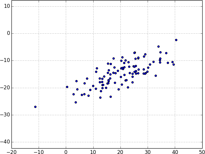
Figure 10-6. Data with the “wrong” axes

Most of the variation in the data seems to be along a single dimension that doesn’t correspond to either the x-axis or the y-axis.

When this is the case, we can use a technique called principal component analysis (PCA) to extract one or more dimensions that capture as much of the variation in the data as possible.

Note

In practice, you wouldn’t use this technique on such a low-dimensional dataset. Dimensionality reduction is mostly useful when your dataset has a large number of dimensions and you want to find a small subset that captures most of the variation. Unfortunately, that case is difficult to illustrate in a two-dimensional book format.

As a first step, we’ll need to translate the data so that each dimension has mean 0:

from scratch.linear_algebra import subtract

def de_mean(data: List[Vector]) -> List[Vector]:
    """Recenters the data to have mean 0 in every dimension"""
    mean = vector_mean(data)
    return [subtract(vector, mean) for vector in data]

(If we don’t do this, our techniques are likely to identify the mean itself rather than the variation in the data.)

Figure 10-7 shows the example data after de-meaning.

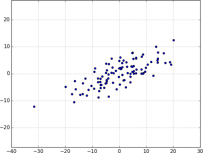
Figure 10-7. Data after de-meaning

Now, given a de-meaned matrix X, we can ask which is the direction that captures the greatest variance in the data.

Specifically, given a direction d (a vector of magnitude 1), each row x in the matrix extends dot(x, d) in the d direction. And every nonzero vector w determines a direction if we rescale it to have magnitude 1:

from scratch.linear_algebra import magnitude

def direction(w: Vector) -> Vector:
    mag = magnitude(w)
    return [w_i / mag for w_i in w]

Therefore, given a nonzero vector w, we can compute the variance of our dataset in the direction determined by w:

from scratch.linear_algebra import dot

def directional_variance(data: List[Vector], w: Vector) -> float:
    """
    Returns the variance of x in the direction of w
    """
    w_dir = direction(w)
    return sum(dot(v, w_dir) ** 2 for v in data)

We’d like to find the direction that maximizes this variance. We can do this using gradient descent, as soon as we have the gradient function:

def directional_variance_gradient(data: List[Vector], w: Vector) -> Vector:
    """
    The gradient of directional variance with respect to w
    """
    w_dir = direction(w)
    return [sum(2 * dot(v, w_dir) * v[i] for v in data)
            for i in range(len(w))]

And now the first principal component that we have is just the direction that maximizes the directional_variance function:

from scratch.gradient_descent import gradient_step

def first_principal_component(data: List[Vector],
                              n: int = 100,
                              step_size: float = 0.1) -> Vector:
    # Start with a random guess
    guess = [1.0 for _ in data[0]]

    with tqdm.trange(n) as t:
        for _ in t:
            dv = directional_variance(data, guess)
            gradient = directional_variance_gradient(data, guess)
            guess = gradient_step(guess, gradient, step_size)
            t.set_description(f"dv: {dv:.3f}")

    return direction(guess)

On the de-meaned dataset, this returns the direction [0.924, 0.383], which does appear to capture the primary axis along which our data varies (Figure 10-8).

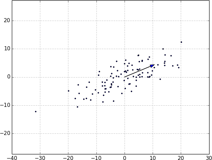
Figure 10-8. First principal component

Once we’ve found the direction that’s the first principal component, we can project our data onto it to find the values of that component:

from scratch.linear_algebra import scalar_multiply

def project(v: Vector, w: Vector) -> Vector:
    """return the projection of v onto the direction w"""
    projection_length = dot(v, w)
    return scalar_multiply(projection_length, w)

If we want to find further components, we first remove the projections from the data:

from scratch.linear_algebra import subtract

def remove_projection_from_vector(v: Vector, w: Vector) -> Vector:
    """projects v onto w and subtracts the result from v"""
    return subtract(v, project(v, w))

def remove_projection(data: List[Vector], w: Vector) -> List[Vector]:
    return [remove_projection_from_vector(v, w) for v in data]

Because this example dataset is only two-dimensional, after we remove the first component, what’s left will be effectively one-dimensional (Figure 10-9).

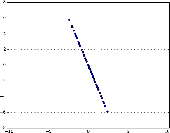
Figure 10-9. Data after removing the first principal component

At that point, we can find the next principal component by repeating the process on the result of remove_projection (Figure 10-10).

On a higher-dimensional dataset, we can iteratively find as many components as we want:

def pca(data: List[Vector], num_components: int) -> List[Vector]:
    components: List[Vector] = []
    for _ in range(num_components):
        component = first_principal_component(data)
        components.append(component)
        data = remove_projection(data, component)

    return components

We can then transform our data into the lower-dimensional space spanned by the components:

def transform_vector(v: Vector, components: List[Vector]) -> Vector:
    return [dot(v, w) for w in components]

def transform(data: List[Vector], components: List[Vector]) -> List[Vector]:
    return [transform_vector(v, components) for v in data]

This technique is valuable for a couple of reasons. First, it can help us clean our data by eliminating noise dimensions and consolidating highly correlated dimensions.

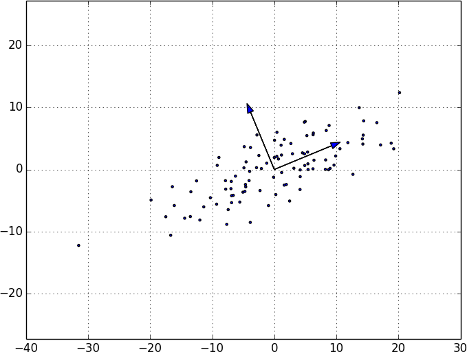
Figure 10-10. First two principal components

Second, after extracting a low-dimensional representation of our data, we can use a variety of techniques that don’t work as well on high-dimensional data. We’ll see examples of such techniques throughout the book.

At the same time, while this technique can help you build better models, it can also make those models harder to interpret. It’s easy to understand conclusions like “every extra year of experience adds an average of $10k in salary.” It’s much harder to make sense of “every increase of 0.1 in the third principal component adds an average of $10k in salary.”

For Further Exploration

• As mentioned at the end of Chapter 9, pandas is probably the primary Python tool for cleaning, munging, manipulating, and working with data. All the examples we did by hand in this chapter could be done much more simply using pandas. Python for Data Analysis (O’Reilly), by Wes McKinney, is probably the best way to learn pandas.

• scikit-learn has a wide variety of matrix decomposition functions, including PCA.