Chapter 14. Simple Linear Regression
Art, like morality, consists in drawing the line somewhere.
G. K. Chesterton
In Chapter 5, we used the correlation function to measure the strength of the linear relationship between two variables. For most applications, knowing that such a linear relationship exists isn’t enough. We’ll want to understand the nature of the relationship. This is where we’ll use simple linear regression.
The Model
Recall that we were investigating the relationship between a DataSciencester user’s number of friends and the amount of time the user spends on the site each day. Let’s assume that you’ve convinced yourself that having more friends causes people to spend more time on the site, rather than one of the alternative explanations we discussed.
The VP of Engagement asks you to build a model describing this relationship. Since you found a pretty strong linear relationship, a natural place to start is a linear model.
In particular, you hypothesize that there are constants α (alpha) and β (beta) such that:
where is the number of minutes user i spends on the site daily, is the number of friends user i has, and ε is a (hopefully small) error term representing the fact that there are other factors not accounted for by this simple model.
Assuming we’ve determined such an alpha and beta, then we make predictions simply with:
defpredict(alpha:float,beta:float,x_i:float)->float:returnbeta*x_i+alpha
How do we choose alpha and beta? Well, any choice of alpha and beta
gives us a predicted output for each input x_i.
Since we know the actual output y_i, we can compute the error for each pair:
deferror(alpha:float,beta:float,x_i:float,y_i:float)->float:"""The error from predicting beta * x_i + alphawhen the actual value is y_i"""returnpredict(alpha,beta,x_i)-y_i
What we’d really like to know is the total error
over the entire dataset.
But we don’t want to just add the errors—if the prediction for x_1 is too high
and the prediction for x_2 is too low, the errors may just cancel out.
So instead we add up the squared errors:
fromscratch.linear_algebraimportVectordefsum_of_sqerrors(alpha:float,beta:float,x:Vector,y:Vector)->float:returnsum(error(alpha,beta,x_i,y_i)**2forx_i,y_iinzip(x,y))
The least squares solution is to
choose the alpha and beta that make sum_of_sqerrors
as small as possible.
Using calculus (or tedious algebra), the error-minimizing alpha and beta are given by:
fromtypingimportTuplefromscratch.linear_algebraimportVectorfromscratch.statisticsimportcorrelation,standard_deviation,meandefleast_squares_fit(x:Vector,y:Vector)->Tuple[float,float]:"""Given two vectors x and y,find the least-squares values of alpha and beta"""beta=correlation(x,y)*standard_deviation(y)/standard_deviation(x)alpha=mean(y)-beta*mean(x)returnalpha,beta
Without going through the exact mathematics, let’s think about why this might be a reasonable solution. The choice of alpha simply says that when we see the average value of the independent variable x, we predict the average value of the dependent variable y.
The choice of beta means that when the input value increases by standard_deviation(x), the prediction then increases by correlation(x, y) * standard_deviation(y). In the case where x and y are perfectly correlated, a one-standard-deviation increase in x results in a one-standard-deviation-of-y increase in the prediction. When they’re perfectly anticorrelated, the increase in x results in a decrease in the prediction. And when the correlation is 0, beta is 0, which means that changes in x don’t affect the prediction at all.
As usual, let’s write a quick test for this:
x=[iforiinrange(-100,110,10)]y=[3*i-5foriinx]# Should find that y = 3x - 5assertleast_squares_fit(x,y)==(-5,3)
Now it’s easy to apply this to the outlierless data from Chapter 5:
fromscratch.statisticsimportnum_friends_good,daily_minutes_goodalpha,beta=least_squares_fit(num_friends_good,daily_minutes_good)assert22.9<alpha<23.0assert0.9<beta<0.905
This gives values of alpha = 22.95 and beta = 0.903. So our model says that we expect a user with n friends to spend 22.95 + n * 0.903 minutes on the site each day. That is, we predict that a user with no friends on DataSciencester would still spend about 23 minutes a day on the site. And for each additional friend, we expect a user to spend almost a minute more on the site each day.
In Figure 14-1, we plot the prediction line to get a sense of how well the model fits the observed data.
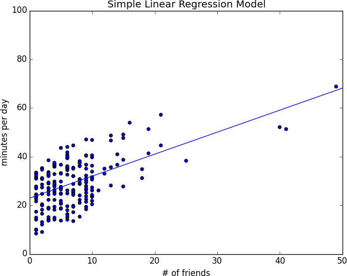
Figure 14-1. Our simple linear model
Of course, we need a better way to figure out how well we’ve fit the data than staring at the graph. A common measure is the coefficient of determination (or R-squared), which measures the fraction of the total variation in the dependent variable that is captured by the model:
fromscratch.statisticsimportde_meandeftotal_sum_of_squares(y:Vector)->float:"""the total squared variation of y_i's from their mean"""returnsum(v**2forvinde_mean(y))defr_squared(alpha:float,beta:float,x:Vector,y:Vector)->float:"""the fraction of variation in y captured by the model, which equals1 - the fraction of variation in y not captured by the model"""return1.0-(sum_of_sqerrors(alpha,beta,x,y)/total_sum_of_squares(y))rsq=r_squared(alpha,beta,num_friends_good,daily_minutes_good)assert0.328<rsq<0.330
Recall that we chose the alpha and beta that minimized the sum of the squared prediction errors. A linear model we could have chosen is “always predict mean(y)” (corresponding to alpha = mean(y) and beta = 0), whose sum of squared errors exactly equals its total sum of squares. This means an R-squared of 0, which indicates a model that (obviously, in this case) performs no better than just predicting the mean.
Clearly, the least squares model must be at least as good as that one, which means that the sum of the squared errors is at most the total sum of squares, which means that the R-squared must be at least 0. And the sum of squared errors must be at least 0, which means that the R-squared can be at most 1.
The higher the number, the better our model fits the data. Here we calculate an R-squared of 0.329, which tells us that our model is only sort of okay at fitting the data, and that clearly there are other factors at play.
Using Gradient Descent
If we write theta = [alpha, beta], we can also solve this using gradient descent:
importrandomimporttqdmfromscratch.gradient_descentimportgradient_stepnum_epochs=10000random.seed(0)guess=[random.random(),random.random()]# choose random value to startlearning_rate=0.00001withtqdm.trange(num_epochs)ast:for_int:alpha,beta=guess# Partial derivative of loss with respect to alphagrad_a=sum(2*error(alpha,beta,x_i,y_i)forx_i,y_iinzip(num_friends_good,daily_minutes_good))# Partial derivative of loss with respect to betagrad_b=sum(2*error(alpha,beta,x_i,y_i)*x_iforx_i,y_iinzip(num_friends_good,daily_minutes_good))# Compute loss to stick in the tqdm descriptionloss=sum_of_sqerrors(alpha,beta,num_friends_good,daily_minutes_good)t.set_description(f"loss: {loss:.3f}")# Finally, update the guessguess=gradient_step(guess,[grad_a,grad_b],-learning_rate)# We should get pretty much the same results:alpha,beta=guessassert22.9<alpha<23.0assert0.9<beta<0.905
If you run this you’ll get the same values for alpha and beta
as we did using the exact formula.
Maximum Likelihood Estimation
Why choose least squares? One justification involves maximum likelihood estimation. Imagine that we have a sample of data that comes from a distribution that depends on some unknown parameter θ (theta):
If we didn’t know θ, we could turn around and think of this quantity as the likelihood of θ given the sample:
Under this approach, the most likely θ is the value that maximizes this likelihood function—that is, the value that makes the observed data the most probable. In the case of a continuous distribution, in which we have a probability distribution function rather than a probability mass function, we can do the same thing.
Back to regression. One assumption that’s often made about the simple regression model is that the regression errors are normally distributed with mean 0 and some (known) standard deviation σ. If that’s the case, then the likelihood based on seeing a pair (x_i, y_i) is:
The likelihood based on the entire dataset is the product of the individual likelihoods, which
is largest precisely when alpha and beta are chosen to minimize the sum of squared errors. That is, in this case (with these assumptions), minimizing the sum of squared errors is equivalent to maximizing the likelihood of the observed data.
For Further Exploration
Continue reading about multiple regression in Chapter 15!